Tales From A Lazy Fat DBA

Its all about Databases, their performance, troubleshooting & much more …. ¯\_(ツ)_/¯

Posts Tagged ‘SQL’

Reading MySQL execution plans without guessing

Posted by FatDBA on July 12, 2026

Every DBA hits this situation eventually. A query that ran in 40 milliseconds last month now takes eleven minutes, nobody deployed anything, and the developer swears the table “isn’t even that big.” The instinct is to add an index and hope. That works often enough to be genuinely dangerous, because it teaches you nothing about why it worked, and the next time the same trick will quietly fail.

The alternative is to read what the optimizer is actually telling you. MySQL is not shy about it. It will hand you its plan, its estimates, and since 8.0.18 .. its real measured execution, if you know how to ask.

Everything below was run on MySQL 8.0.46 against a schema I built specifically to misbehave: 200,000 customers and 1,000,000 orders, with a status column that is dangerously skewed.

CREATE TABLE customers (
  id           INT UNSIGNED NOT NULL AUTO_INCREMENT,
  email        VARCHAR(120) NOT NULL,
  country      CHAR(2)      NOT NULL,
  signup_date  DATE         NOT NULL,
  PRIMARY KEY (id),
  UNIQUE KEY uq_email (email),
  KEY ix_country (country)
) ENGINE=InnoDB;

CREATE TABLE orders (
  id           BIGINT UNSIGNED NOT NULL AUTO_INCREMENT,
  customer_id  INT UNSIGNED    NOT NULL,
  status       VARCHAR(12)     NOT NULL,
  amount       DECIMAL(10,2)   NOT NULL,
  created_at   DATETIME        NOT NULL,
  PRIMARY KEY (id),
  KEY ix_customer (customer_id),
  KEY ix_status (status)
) ENGINE=InnoDB;


-- The skew is the whole point:

status      rows_actual   pct
shipped        980123    98.012
pending         12043     1.204
cancelled        4876     0.488
refunded         2958     0.296

Now comes the main topic of discussion, How the optimizer picks the plan ?

MySQL’s optimizer is cost-based, and the machinery is simpler than people assume. There’s no plan cache learning from history, no adaptive feedback loop. Every compilation is a fresh search over possible strategies, and the cheapest estimated plan wins. Before it costs anything, MySQL rewrites the query. Constants get folded (price > 10 * 5 becomes price > 50). Constants get propagated — if you write WHERE a.id = 42 AND a.id = b.a_id, MySQL infers b.a_id = 42 and pushes that predicate straight into b. Simple views get merged into the outer query. And — this one bites people constantly .. an outer join gets silently converted to an inner join if the WHERE clause rejects NULLs on the inner table. Write LEFT JOIN orders o ... WHERE o.status = 'shipped' and you have written an inner join, whether you meant to or not, because a NULL o.status can never equal 'shipped'.

Then comes range analysis, and this is the part that matters most for the rest of this post. For each usable index, MySQL doesn’t just consult stored statistics. It performs an actual B tree search .. records_in_range() .. physically walking into the index to count how many rows fall inside your predicate’s range. This is real work, touching real pages, at plan time.

Join ordering is a greedy search, not exhaustive. Two conditions govern it: optimizer_search_depth (default 62) and optimizer_prune_level (default 1). For three or four tables MySQL will find something near optimal. For fifteen tables it will find a plan, and that plan may be mediocre. Counterintuitively, if you’re joining that many tables and getting bad plans, lowering optimizer_search_depth to 4 or 8 often produces better plans faster, because you stop the optimizer from burning its budget on a search space it can’t cover anyway.

Costs are computed from tunable constants in mysql.server_cost and mysql.engine_cost …. row_evaluate_cost, io_block_read_cost, and friends. You can change them. You almost definately shouldn’t.

Next lets talk about plan generation and tools we have –> Three tools, three different jobs, and people conflate them constantly.

EXPLAIN gives you the plan as a flat table. It does not run the query. It’s fast, it’s compact, and it’s what you reach for 90% of the time. EXPLAIN FORMAT=JSON gives you the same plan with everything EXPLAIN had to leave out .. the actual cost numbers, which key parts were used, which columns get read, and the exact condition attached to each table. Still doesn’t run the query. When EXPLAIN says something confusing, this is where you go to find out why. EXPLAIN ANALYZE (8.0.18+) actually executes the query and reports what really happened alongside what was predicted. This is the one that ends arguments. It’s also the one you should think twice about before running against production on a DELETE— though for SELECTs it’s just a query that costs you its own runtime.

Same query, all three.

mysql> EXPLAIN SELECT c.email, o.amount FROM customers c
    ->   JOIN orders o ON o.customer_id = c.id
    ->  WHERE o.status = 'refunded' AND c.country = 'JP'\G
*************************** 1. row ***************************
           id: 1
  select_type: SIMPLE
        table: o
         type: ref
possible_keys: ix_customer,ix_status
          key: ix_status
      key_len: 50
          ref: const
         rows: 2958
     filtered: 100.00
        Extra: NULL
*************************** 2. row ***************************
           id: 1
  select_type: SIMPLE
        table: c
         type: eq_ref
possible_keys: PRIMARY,ix_country
          key: PRIMARY
      key_len: 4
          ref: shop.o.customer_id
         rows: 1
     filtered: 5.00
        Extra: Using where


-- JSON format adds the details what were hidden
{
  "query_block": {
    "cost_info": { "query_cost": "3665.19" },
    "nested_loop": [
      { "table": {
          "table_name": "o",
          "access_type": "ref",
          "key": "ix_status",
          "used_key_parts": ["status"],
          "key_length": "50",
          "rows_examined_per_scan": 2958,
          "rows_produced_per_join": 2958,
          "filtered": "100.00",
          "cost_info": { "read_cost": "829.74", "eval_cost": "295.80",
                         "prefix_cost": "1125.54" }
      }},
      { "table": {
          "table_name": "c",
          "access_type": "eq_ref",
          "key": "PRIMARY",
          "key_length": "4",
          "ref": ["shop.o.customer_id"],
          "rows_examined_per_scan": 1,
          "rows_produced_per_join": 147,
          "filtered": "5.00",
          "cost_info": { "prefix_cost": "3665.19" },
          "attached_condition": "(`shop`.`c`.`country` = 'JP')"
      }}
    ]
  }
}

prefix_cost is cumulative … 1125.54 after the first table, 3665.19 after both. rows_produced_per_join: 147 is the estimate flowing out of the join. attached_condition shows you exactly what’s being evaluated where, which is worth the verbosity all by itself. And now comes the truth time 🙂

mysql> EXPLAIN ANALYZE SELECT c.email, o.amount FROM customers c
    ->   JOIN orders o ON o.customer_id = c.id
    ->  WHERE o.status = 'refunded' AND c.country = 'JP'\G

-> Nested loop inner join  (cost=4286 rows=148) (actual time=1.18..37.4 rows=56 loops=1)
    -> Index lookup on o using ix_status (status='refunded')
         (cost=1035 rows=2958) (actual time=0.826..11.5 rows=2958 loops=1)
    -> Filter: (c.country = 'JP')
         (cost=0.999 rows=0.05) (actual time=0.00866..0.00866 rows=0.0189 loops=2958)
        -> Single-row index lookup on c using PRIMARY (id=o.customer_id)
             (cost=0.999 rows=1) (actual time=0.00842..0.00844 rows=1 loops=2958)

Read that inner block carefully, because it’s the single most misread thing in MySQL. rows=0.0189 loops=2958 does not mean MySQL found 0.0189 rows. It means the inner side was executed 2,958 times, and averaged 0.0189 rows per execution. Multiply: 0.0189 × 2958 ≈ 56, which is exactly the final row count. Same for timing … actual time=0.00866 is per loop, not total. The total time for that operation is roughly 0.00866 × 2958 ≈ 25ms. Estimated 148 rows, got 56. That’s a 2.6× overestimate, and I’ll come back to where it came from.

Next, lets check all of the columns and values used in the plan and what exact that means..

id : which SELECT this row belongs to. Same number across rows means same query block, and the order those rows appear in is the join order. Different numbers mean subqueries or unions, and a bigger id executes first.

select_type : SIMPLE for a plain query, PRIMARY for the outer part of one with subqueries, SUBQUERY, DERIVED, UNION, MATERIALIZED. If you see DEPENDENT SUBQUERY, tense up: it means the subquery reruns for every outer row.

table : the table, or a synthetic name like <derived2> for a derived table.

type : The access method. Most important column in the output; full section below.

possible_keys : indexes the optimizer considered. NULL here is diagnostic: it means no index could even theoretically serve this predicate, so before you tune anything, go look at whether the right index exists at all.

key : what it actually chose. When possible_keys lists three indexes and key picks one, the other two lost on cost. That’s a decision you can second-guess.

key_len : bytes of the index actually used. This is the column that catches partial index usage, and people ignore it because the calculation/maths looks like magic, but It isn’t:

  • Each column’s base size (INT = 4, BIGINT = 8)
  • +1 byte if the column is NULLable
  • For variable-length strings, +2 bytes for the length prefix
  • Character columns are counted in bytes, not characters — under utf8mb4 that’s 4 bytes per character

Check it against our real output. status is VARCHAR(12) NOT NULL under utf8mb4: 12 × 4 = 48 octets, no null byte, +2 for the length prefix = 50. And EXPLAIN reports key_len: 50. Exactly. ix_country on CHAR(2) gives 2 × 4 = 8, and yes, key_len: 8.

I built a throwaway table to prove the NULL byte is real …

INT NULL      -> key_len: 5     (4 + 1 null byte)
INT NOT NULL  -> key_len: 4
VARCHAR(10) NULL -> key_len: 43 (10*4 + 1 + 2)

Why care? Because on a composite index (a, b, c), key_len tells you how many of those columns are actually doing work. If key_len only accounts for a, then b and c are dead weight for this query and you’ve been fooling yourself about your index.

ref : what’s being compared against the indexed column. const for a literal, or a column name like shop.o.customer_id when the value comes from an earlier table in the join. This is how you read the data flow of a nested loop.

rows : estimated rows examined for this step. Estimated, and in a join it’s per iteration, not total.

filtered : percentage of those rows expected to survive the WHERE conditions that weren’t handled by the index. This is the column everyone skips and shouldn’t, because rows × filtered / 100 is what actually flows to the next table. In the join above, table c shows rows: 1, filtered: 5.00 … MySQL believes 5% of customers are in Japan. It isn’t 5%. There are eight countries in my data and JP is the rarest at about 2%. That 5.00 is a guess, and it’s precisely why the join estimate came out at 148 instead of 56.

Extra — everything else, and where the real diagnoses live.

Access types, which is best and the worst ??

const : at most one row, matched on a primary key or unique index against a literal. MySQL reads it once during optimization and substitutes it as a constant. You cannot do better.

EXPLAIN SELECT email FROM customers WHERE id = 42;
type: const   key: PRIMARY   key_len: 4   ref: const   rows: 1

eq_ref : one row from this table per row from the previous table, via PK or unique index. This is the ideal for the driven side of a join, and it’s what our join got:

type: eq_ref   key: PRIMARY   key_len: 4   ref: shop.o.customer_id   rows: 1

ref : A non-unique index lookup, may return many rows. Perfectly healthy. Our status='refunded' lookup is ref with rows: 2958.

range : index scan over a bounded range. BETWEEN, >, IN (...), LIKE 'foo%'.

EXPLAIN SELECT id FROM orders WHERE id BETWEEN 100 AND 500;
type: range   key: PRIMARY   key_len: 8   rows: 401   Extra: Using where; Using index

401 estimated, 401 actual. B-tree dives are good at this.

index : full scan of the entire index. Not a lookup. It’s ALL wearing a nicer coat, and it’s only cheap because the index is narrower than the table:

EXPLAIN SELECT COUNT(country) FROM customers;
type: index   key: ix_country   rows: 199488   Extra: Using index

ALL : Is a full table scan. Every row, from disk.

EXPLAIN SELECT * FROM orders WHERE amount > 500;
type: ALL   possible_keys: NULL   key: NULL   rows: 997152   filtered: 33.33

Note: possible_keys: NULL : there’s no index on amount, so this was never even a contest. And note rows: 997152 when the table holds exactly 1,000,000 rows. InnoDB’s row count is itself an estimate, sampled, not counted. Don’t trust it to the digit. A full scan is not automatically a bug, by the way. If you’re reading 98% of the table, a scan genuinely is cheaper than a million index lookups each followed by a random row fetch. The bug is a full scan on a selective predicate.

Now lets read ‘EXTRA’:

Using index : a covering index. Everything the query needs lives in the index; the table itself is never touched. This is the single biggest win available in the Extra column, and it’s easy to engineer. Watch this ..

-- before
EXPLAIN SELECT customer_id, status FROM orders WHERE status='refunded';
type: ref   key: ix_status   rows: 2958   Extra: NULL

ALTER TABLE orders ADD INDEX ix_status_cust (status, customer_id);

-- after
type: ref   key: ix_status_cust   rows: 2958   Extra: Using index

Same rows, same access type, but Extra flipped to Using index and we eliminated 2,958 random primary-key lookups.

Using where : MySQL is filtering rows after fetching them from the storage engine. Not fatal on its own. But Using where sitting next to type: ALL and a low filtered is the classic missing-index signature.

Using index condition : Index Condition Pushdown. Different from Using index, and the names are unhelpfully similar. ICP means the condition is evaluated at the index level so non-matching entries never trigger a row fetch. It’s a real optimization, not a warning.

Using temporary : an internal temp table was built, usually for GROUP BY or DISTINCT. In 8.0 it’s TempTable in memory up to temptable_max_ram (default 1GB), then spills to disk. Small ones are fine. Big ones are why your query fell off a cliff.

Using filesort : the results had to be sorted, because no index provided the required order. “Filesort” does not mean it hit disk; it may well sort entirely in memory within sort_buffer_size. Bad name, causes endless confusion. Still, it’s work you might be able to design away with the right index.

Both at once, which is the combination worth hunting for:

EXPLAIN SELECT c.country, SUM(o.amount) t
  FROM customers c JOIN orders o ON o.customer_id = c.id
 WHERE o.status = 'pending'
 GROUP BY c.country ORDER BY t DESC;

table: o   type: ref   key: ix_status   rows: 22536
Extra: Using temporary; Using filesort

The GROUP BY builds the temp table, and the ORDER BY SUM(o.amount) forces the filesort on top of it .. you cannot index your way out of ordering by an aggregate that doesn’t exist until the group is computed. Sometimes the answer is “this is inherent, accept it.” Knowing which it is, is the job.

Scenario one: the cardinality trap (and where the usual advice is wrong)

Here’s where I have to correct something I’ve written myself in the past.

The standard story goes: MySQL assumes uniform distribution, so on a skewed column it wildly misestimates, and histograms fix it. Let’s test that. Two queries, same column, wildly different selectivity:

-- refunded: 2,958 rows, 0.296% of table
type: ref   key: ix_status   rows: 2958   filtered: 100.00

-- shipped: 980,123 rows, 98% of table
type: ref   key: ix_status   rows: 498576   filtered: 100.00

For refunded, rows: 2958 :: the exact true count. Not close. Exact. So much for uniform-distribution assumptions. This is records_in_range() diving into the B-tree and counting for real. But look at shipped: estimated 498,576, and EXPLAIN ANALYZE reports the truth:

-> Index lookup on orders using ix_status (status='shipped')
   (cost=52812 rows=498576) (actual time=2.35..2136 rows=980123 loops=1)

980,123 actual against 498,576 estimated. A 1.97× underestimate … on the unselective value, not the selective one. The dive samples a bounded number of pages; over a huge range it extrapolates, and extrapolation drifts. So, surely a histogram fixes it?

ANALYZE TABLE orders UPDATE HISTOGRAM ON status WITH 16 BUCKETS;
-- re-run, WITH histogram in place
type: ref   key: ix_status   rows: 498576   filtered: 100.00

Nothing changed. Identical estimate. This is the finding I did not expect, and it’s the most useful thing in this post: when a usable index exists, the index dive wins and the histogram is ignored for the rows estimate.m Histograms feed filtered, not rows. To see them work, take the index away:

-- ix_status dropped
type: ALL   possible_keys: NULL   rows: 997152   filtered: 0.30   Extra: Using where

-> Filter: (orders.status = 'refunded')  (cost=100912 rows=2949)
   (actual time=0.83..251 rows=2958 loops=1)
    -> Table scan on orders  (cost=100912 rows=997152)
       (actual time=0.738..200 rows=1e+6 loops=1)

filtered: 0.30 against a true 0.296%. Estimated 2,949 rows, actual 2,958. The histogram is superb — but only where the optimizer had nothing better.

The practical rule, then, is the opposite of the folklore. Build histograms on columns you are filtering on but have not indexed … typically because they’re low-cardinality and an index would be pointless, but they still need a decent filtered estimate to drive join ordering. Indexing the column and histogramming it is mostly wasted effort. One more trap while we’re in here. Look at the stored histogram:

"buckets": [
  ["base64:type254:Y2FuY2VsbGVk", 0.004594302009347028],
  ["base64:type254:cGVuZGluZw==",  0.01689858210334539],
  ["base64:type254:cmVmdW5kZWQ=",  0.019855833971430835],
  ["base64:type254:c2hpcHBlZA==",  1.0]
],
"histogram-type": "singleton",
"sampling-rate": 0.07373942163752957

Those are cumulative frequencies, not per-value. refunded is not 1.98% of the table … it’s 0.0199 − 0.0169 = 0.0030, i.e. 0.30%. The per-value frequency is the difference between consecutive buckets. I have watched people read that 1.0 on shipped and conclude the histogram is broken. And while we’re looking at bad statistics, check what InnoDB thinks ix_status contains:

INDEX_NAME    COLUMN_NAME    CARDINALITY
ix_status     status         3
ix_customer   customer_id    197646
PRIMARY       id             997152

Cardinality 3. There are four distinct statuses. The default 20 page sample (innodb_stats_persistent_sample_pages) missed one entirely. If you have a low-cardinality column with a rare value that matters, raise that setting for the table and re-analyze … otherwise the optimizer is reasoning about a value it doesn’t know exists.

Scenario two: join order, and why it’s the whole game

Nested-loop joins have a brutal asymmetry: the driving table’s row count becomes the loop count for everything after it. Get it backwards and you multiply your own pain. MySQL got our join right. It drove from orders (2,958 refunded rows) and probed customers by primary key:

-> Nested loop inner join  (cost=4286 rows=148) (actual time=1.18..37.4 rows=56 loops=1)
    -> Index lookup on o using ix_status (status='refunded')
         (cost=1035 rows=2958) (actual ... rows=2958 loops=1)
    -> Filter: (c.country = 'JP')
         (cost=0.999 rows=0.05) (actual ... rows=0.0189 loops=2958)

2,958 loops. 37.4ms. …. Now let’s force the mistake with STRAIGHT_JOIN, which pins join order to the order you wrote:

-> Nested loop inner join  (cost=7692 rows=202) (actual time=1.2..93.1 rows=56 loops=1)
    -> Index lookup on c using ix_country (country='JP')
         (cost=920 rows=4039) (actual ... rows=4039 loops=1)
    -> Filter: (o.status = 'refunded')
         (cost=1.2 rows=0.05) (actual ... rows=0.0139 loops=4039)
        -> Index lookup on o using ix_customer (customer_id=c.id)
             (cost=1.2 rows=4.79) (actual ... rows=5.03 loops=4039)

4,039 loops. 93.1ms. Identical 56 rows out, two and a half times the time. And the inner side is worse than the loop count suggests: each of those 4,039 loops now fetches ~5 orders and throws nearly all of them away (rows=5.03 in, rows=0.0139 surviving the filter). We’re reading roughly 20,000 order rows to keep 56.

The optimizer picked correctly here. It doesn’t always … and when it doesn’t, the reason is almost always upstream: a filtered percentage built on a guess. Recall that filtered: 5.00 on customers. MySQL had no histogram on country, so it fell back to a canned guess, and that guess is what produced the 148-row estimate against 56 actual. On this query the error was harmless. On a five-table join, an error like that at step one compounds through every subsequent step, and that is how you get a plan that’s wrong by four orders of magnitude. While we’re here: filtered: 33.33 on the amount > 500 scan earlier is the same phenomenon in its purest form. That number is not measured. It’s MySQL’s hardcoded 1/3 guess for a range condition on a column it knows nothing about. Any time you see 33.33, 11.11, or 5.00 in filtered, you are looking at a guess, not a statistic.

Selecting and validating indexes

Start with the predicate, not the query text. Equality columns go first in a composite index, then range columns, then columns needed only for ORDER BY or covering. The reason is mechanical: a B tree can only use one range column before the ordering breaks down for everything to its right.

Check key_len to confirm the index is being used as far as you think it is. If your index is (status, customer_id, created_at) and key_len comes back as 50, only status is doing work.

Aim for Using index in Extra where you can. Adding one column to an existing index to make it covering is often a bigger win than adding a whole new index … and it costs you far less on write throughput.

Then validate with EXPLAIN ANALYZE, and compare estimated against actual. A ratio inside about 10× is usually fine. Beyond that, ask why: stale stats (run ANALYZE TABLE), a sample too small to see your rare values (raise innodb_stats_persistent_sample_pages), or a filtered built on a guess (histogram the column … as long as it isn’t already indexed).

Finally, resist the urge to just add the index. Every index is a write tax on every INSERT, UPDATE, and DELETE against that table, forever. Before you create one, check sys.schema_unused_indexes and sys.schema_redundant_indexes … I have never once run those on a mature production system and not found something to drop.

So, in short, summary, EXPLAIN tells you the plan. FORMAT=JSON tells you the costs behind it. EXPLAIN ANALYZE tells you the truth, and the truth is the only one of the three you can act on with confidence. Read rows and filtered together, always, because rows × filtered / 100 is what actually flows downstream. Treat loops as a multiplier, and remember that rows= and actual time= on an inner node are per loop. And when filtered shows you 33.33 or 5.00, recognise it for what it is: MySQL shrugging.

Then go and check whether the optimizer’s guess matched reality. Usually it does. The eleven-second query is where it didn’t.

Hope It Helped!
Prashant Dixit

Posted in Uncategorized | Tagged: , , , | Leave a Comment »

fatdba explores Vector Search in Oracle 23ai

Posted by FatDBA on July 23, 2025

So Oracle rolled out 23ai a while back and like every major release, it came packed with some really cool and interesting features. One that definitely caught my eye was Vector Search. I couldn’t resist diving in… and recently I explored it in depth and would like to share a though on this subject.

You see, we’ve been doing LIKE '%tax policy%' since forever. But now, Oracle’s SQL has become more powerful. Not only does it match words … it matches meaning.

So here’s me trying to explain what vector search is, how Oracle does it, why you’d care, and some examples that’ll hopefully make it click.

What’s Vector Search, Anyway?

Alright, imagine this:

You have a table of products. You search for “lightweight laptop for travel”.
Some entries say “ultrabook”, others say “portable notebook”, and none mention “lightweight” or “travel”. Old-school SQL would’ve said: “No Matches Found”

But with vector search, it gets it. Oracle turns all that text into math .. basically, a long list of numbers called a vector … and compares meanings instead of words.

So What’s a Vector?

When we say “vector” in vector search, we’re not talking about geometry class. In the world of AI and databases, a vector is just a long list of numbers … each number representing some aspect or feature of the original input (like a sentence, product description, image, etc.).

Here’s a basic example:
[0.12, -0.45, 0.88, …, 0.03]
This is a vector … maybe a 512 or 1536-dimension one .. depending on the embedding model used (like OpenAI, Oracle’s built-in model, Cohere, etc.).

Each number in this list is abstract, but together they represent the essence or meaning of your data.

Let’s say you have these two phrases:
“Apple is a tech company”
“iPhone maker based in California”

Now, even though they don’t share many words, they mean nearly the same thing. When passed through an embedding model, both phrases are converted into vectors:

Vector A: [0.21, -0.32, 0.76, …, 0.02]
Vector B: [0.22, -0.30, 0.74, …, 0.01]

They look very close … and that’s exactly the point.

What Oracle 23ai Gives You

  • A new VECTOR datatype (yeah!)
  • AI_VECTOR() function to convert text into vectors
  • VECTOR_INDEX to make search blazing fast
  • VECTOR_DISTANCE() to measure similarity
  • It’s all native in SQL ..no need for another vector DB bolted on

Let’s Build Something Step-by-Step

We’ll build a simple product table and do a vector search on it.

Step 1: Create the table

CREATE TABLE products (
  product_id     NUMBER PRIMARY KEY,
  product_name   VARCHAR2(100),
  description    VARCHAR2(1000),
  embedding      VECTOR(1536)
);

1536? Yeah, that’s the number of dimensions from Oracle’s built-in embedding model. Depends on which one you use.

Step 2: Generate vector embeddings

UPDATE products
SET embedding = ai_vector('text_embedding', description);

This’ll take the description, pass it through Oracle’s AI model, and give you a vector. Magic.

Step 3: Create the vector index

CREATE VECTOR INDEX product_vec_idx
ON products (embedding)
WITH (DISTANCE METRIC COSINE);

This speeds up the similarity comparisons … much like an index does for normal WHERE clauses.

Step 4: Semantic Search in SQL

SELECT product_id, product_name, 
       VECTOR_DISTANCE(embedding, ai_vector('text_embedding', 'light laptop for designers')) AS score
FROM products
ORDER BY score
FETCH FIRST 5 ROWS ONLY;

Now we’re searching for meaning, not words.

VECTOR_DISTANCE Breakdown

You can use different math behind the scenes:

VECTOR_DISTANCE(v1, v2 USING COSINE)
VECTOR_DISTANCE(v1, v2 USING EUCLIDEAN)
VECTOR_DISTANCE(v1, v2 USING DOT_PRODUCT)

Cosine is the usual go-to for text. Oracle handles the rest for you.

Use Cases You’ll Actually Care About

1. Semantic Product Search — “Fast shoes for runners” => shows “Nike Vaporfly”, even if it doesn’t say “fast”.

2. Similar Document Retrieval — Find all NDAs that look like this one (even with totally different words).

3. Customer Ticket Suggestion — Auto-suggest resolutions from past tickets. Saves your support team hours.

4. Content Recommendation — “People who read this also read…” kind of stuff. Easy to build now.

5. Risk or Fraud Pattern Matching — Find transactions that feel like fraud ..even if the details don’t match 1:1.

I know it might sound little confusing .. lets do a Onwe more example : Legal Document Matching

CREATE TABLE legal_docs (
  doc_id       NUMBER PRIMARY KEY,
  title        VARCHAR2(255),
  content      CLOB,
  content_vec  VECTOR(1536)
);

Update vectors:

UPDATE legal_docs
SET content_vec = ai_vector('text_embedding', content);

Now find similar docs:

SELECT doc_id, title
FROM legal_docs
ORDER BY VECTOR_DISTANCE(content_vec, ai_vector('text_embedding', 'confidentiality in government contracts'))
FETCH FIRST 10 ROWS ONLY;

That’s it. You’re officially building an AI-powered legal search engine.

Things to Know

  • Creating vectors can be heavy .. batch it.
  • Indexing speeds up similarity search a lot.
  • Combine with normal filters for best results:
SELECT * FROM products
WHERE category = 'laptop'
ORDER BY VECTOR_DISTANCE(embedding, ai_vector('gaming laptop under 1kg'))
FETCH FIRST 5 ROWS ONLY;

Final Thoughts from fatdba

I’m honestly impressed. Oracle took something that felt like ML black magic and put it right in SQL. No external service. No complicated setups. Just regular SQL, but smater.

Hope It Helped!
Prashant Dixit
Database Architect @RENAPS
Reach us at : https://renaps.com/

Posted in Uncategorized | Tagged: , , , , , , , , , , , , , , | Leave a Comment »

Diagnosing a MySQL database performance Issue Using MySQLTuner.

Posted by FatDBA on July 20, 2025

A few weeks ago, we ran into a pretty nasty performance issue on one of our MySQL production-like grade databases. It started with slow application response times and ended with my phone blowing up with alerts. Something was clearly wrong, and while I suspected some bad queries or config mismatches, I needed a fast way to get visibility into what was really happening under the hood.

This is where MySQLTuner came to the rescue, again 🙂 I’ve used this tool in the past, and honestly, it’s one of those underrated gems for DBAs and sysadmins. It’s a Perl script that inspects your MySQL configuration and runtime status and then gives you a human-readable report with recommendations.

Let me walk you through how I used it to identify and fix the problem ..step by step .. including actual command output, what I changed, and the final outcome.

Step 1: Getting MySQLTuner

First things first, if you don’t already have MySQLTuner installed, just download it:

bashCopyEditwget https://raw.githubusercontent.com/major/MySQLTuner-perl/master/mysqltuner.pl
chmod +x mysqltuner.pl

You don’t need to install anything. Just run it like this:

bashCopyEdit./mysqltuner.pl --user=root --pass='YourStrongPassword'

(Note: Avoid running this in peak traffic hours on prod unless you’re sure about your load and risk.)

Step 2: Sample Output Snapshot

Here’s a portion of what I got when I ran it:

 >>  MySQLTuner 2.6.20 
 >>  Run with '--help' for additional options and output filtering

[OK] Currently running supported MySQL version 5.7.43
[!!] Switch to 64-bit OS - MySQL cannot use more than 2GB of RAM on 32-bit systems
[OK] Operating on 64-bit Linux

-------- Performance Metrics -------------------------------------------------
[--] Up for: 3d 22h 41m  (12M q [35.641 qps], 123K conn, TX: 92G, RX: 8G)
[--] Reads / Writes: 80% / 20%
[--] Binary logging is enabled (GTID MODE: ON)
[--] Total buffers: 3.2G global + 2.8M per thread (200 max threads)
[OK] Maximum reached memory usage: 4.2G (27.12% of installed RAM)
[!!] Slow queries: 15% (1M/12M)
[!!] Highest connection usage: 98% (197/200)
[!!] Aborted connections: 2.8K
[!!] Temporary tables created on disk: 37% (1M on disk / 2.7M total)

-------- MyISAM Metrics ------------------------------------------------------
[!!] Key buffer used: 17.2% (89M used / 512M cache)
[!!] Key buffer size / total MyISAM indexes: 512.0M/800.0M

-------- InnoDB Metrics ------------------------------------------------------
[OK] InnoDB buffer pool / data size: 2.0G/1.5G
[OK] InnoDB buffer pool instances: 1
[--] InnoDB Read buffer efficiency: 99.92% (925M hits / 926M total)
[!!] InnoDB Write log efficiency: 85.10% (232417 hits / 273000 total)
[!!] InnoDB log waits: 28

-------- Recommendations -----------------------------------------------------
General recommendations:
    Control warning line(s) size by reducing joins or increasing packet size
    Increase max_connections slowly if needed
    Reduce or eliminate persistent connections
    Enable the slow query log to troubleshoot bad queries
    Consider increasing the InnoDB log file size
    Query cache is deprecated and should be disabled

Variables to adjust:
    max_connections (> 200)
    key_buffer_size (> 512M)
    innodb_log_file_size (>= 512M)
    tmp_table_size (> 64M)
    max_heap_table_size (> 64M)

Step 3: What I Observed

Here’s what stood out for me:

1. Too many slow queries — 15% of all queries were slow. That’s a huge red flag. This wasn’t being logged properly either — the slow query log was off.

2. Disk-based temporary tables — 37% of temporary tables were being written to disk. This kills performance during joins and sorts.

3. Connections hitting limit — 197 out of 200 max connections used at peak. Close to saturation ..possibly causing application timeouts.

4. MyISAM key buffer inefficient — Key buffer was too small for the amount of MyISAM index data (yes, we still have a couple legacy MyISAM tables..

5. InnoDB log file too small — Frequent log flushing and waits were indicated, meaning innodb_log_file_size wasn’t enough for our write load.

Step 4: Actions I Took

Here’s what I changed based on the output and a quick double-check of our workload patterns:

– Enabled Slow Query Log

sqlCopyEditSET GLOBAL slow_query_log = 'ON';
SET GLOBAL long_query_time = 1;

And updated /etc/my.cnf:

iniCopyEditslow_query_log = 1
slow_query_log_file = /var/log/mysql-slow.log
long_query_time = 1

– Increased tmp_table_size and max_heap_table_size:

iniCopyEdittmp_table_size = 128M
max_heap_table_size = 128M

(This reduced the % of temp tables going to disk.)

– Raised innodb_log_file_size:

iniCopyEditinnodb_log_file_size = 512M
innodb_log_files_in_group = 2

Caution: You need to shut down MySQL cleanly and delete old redo logs before applying this change.

– Raised key_buffer_size:

iniCopyEditkey_buffer_size = 1G

We still had some legacy MyISAM usage and this definitely helped reduce read latency.

– Upped the max_connections a bit (but also discussed with devs about app-level connection pooling):

iniCopyEditmax_connections = 300

Step 5: Post-Change Observations

After making these changes and restarting MySQL (for some of the changes to take effect), here’s what I observed:

  • CPU dropped by ~15% at peak hours.
  • Threads_running dropped significantly, meaning less contention.
  • Temp table usage on disk dropped to 12%.
  • Slow query log started capturing some really bad queries, which were fixed in the app code within a few days.
  • No more aborted connections or connection errors from the app layer.

Final Thoughts

MySQLTuner is not a magic bullet, but it’s one of those tools that gives you quick, actionable insights without the need to install big observability stacks or pay for enterprise APM tools. I’d strongly suggest any MySQL admin or engineer dealing with production performance issues keep this tool handy.

It’s also good for periodic health checks, even if you’re not in a crisis. Run it once a month or so, and you’ll catch slow config drifts or usage pattern changes.

Resources

If you’ve had a similar experience or used MySQLTuner in your infra, would love to hear what kind of findings you had. Drop them in the comments or message me directly .. Want to know more 🙂 Happy tuning!

Hope It Helped!
Prashant Dixit
Database Architect @RENAPS
Reach us at : https://renaps.com/

Posted in Uncategorized | Tagged: , , , , , , , , , | Leave a Comment »

Leveraging SQLT to transfer execution plans between SQL IDs using coe_load_sql_profile.sql

Posted by FatDBA on March 11, 2025

Hi All,

Have you used coe_load_sql_profile.sql before? I mean a lot of people uses coe_xfr_sql_profile.sql from SQLT and these two scripts deals with SQL profiles in Oracle, but their purposes and use cases differ. coe_xfr_sql_profile.sql is used to export and migrate an existing SQL Profile from one system to another, ensuring performance stability across environments. coe_load_sql_profile.sql is used to create a new SQL Profile by capturing the execution plan from a modified SQL query and applying it to the original query, forcing it to use the optimized plan.

Let me first explain a little bit more of the toolkit – Oracle SQLT (SQLTXPLAIN) which is a powerful tool designed to help DBAs analyze and troubleshoot SQL performance issues and all above mentioned scripts are part of the kit provided by Oracle and written by none other than Carlos Sierra.

A common question DBAs encounter is: Can we plug the execution plan of one SQL ID into another SQL ID? …. The answer is YES! This can be accomplished using the SQLT script coe_load_sql_profile.sql. In this blog, we will explore how to use this script to achieve plan stability by enforcing a preferred execution plan across different SQL IDs. It examines the memory and AWR both to look text of the SQL IDs you passed and then it queries GV$SQL_PLAN and DBA_HIST_SQL_PLAN to extract the execution plan hash value from the modified SQL. Once it’s done collecting that information, it performs a loop to extract optimizer hints of the modified SQL’s execution plan. Finally it creates a SQL Profile using DBMS_SQLTUNE.IMPORT_SQL_PROFILE.

Let’s give a quick demo … assume we have two SQL statements:

SQL ID 1: 78a1nbdabcba (Original SQL) …. SQL ID 2: 9na182nn2bnn (Modified SQL)
Both queries are logically similar but produce different execution plans.
Our goal is to take the execution plan from SQL ID 1 and apply it to SQL ID 2.

connect system/monkey123
SQL> @coe_load_sql_profile.sql 
or 
SQL> START coe_load_sql_profile.sql <ORIGINAL_SQL_ID> <MODIFIED_SQL_ID>


Parameter 1:
ORIGINAL_SQL_ID (required)

Enter value for 1: 78a1nbdabcba

Parameter 2:
MODIFIED_SQL_ID (required)

Enter value for 2: 9na182nn2bnn


     PLAN_HASH_VALUE          AVG_ET_SECS
-------------------- --------------------
          1181381381                 .003

Parameter 3:
PLAN_HASH_VALUE (required)

Enter value for 3: 1181381381

Values passed to coe_load_sql_profile:
~~~~~~~~~~~~~~~~~~~~~~~~~~~~~~~~~~~~~
ORIGINAL_SQL_ID: "78a1nbdabcba"
MODIFIED_SQL_ID: "9na182nn2bnn"
PLAN_HASH_VALUE: "1181381381"

.
.
.

ORIGINAL:78a1nbdabcba MODIFIED:9na182nn2bnn PHV:1181381381 SIGNATURE:16731003137917309319 CREATED BY COE_LOAD_SQL_PROFILE.SQL
SQL>SET ECHO OFF;

****************************************************************************
* Enter password to export staging table STGTAB_SQLPROF_78a1nbdabcba
****************************************************************************

Export: Release 19.0.0- Production on Sun Mar 08 14:45:47 2012

Copyright (c) 1982, 2024, Oracle and/or its affiliates.  All rights reserved.

Password:
.
.
.

coe_load_sql_profile completed.


Run original query
SQL> select ename from DIXIT where ename='Name';

Plan hash value: 1181381381

---------------------------------------------------------------
| Id  | Operation         | Name | Rows  | Bytes | Cost (%CPU)| 
---------------------------------------------------------------
|   0 | SELECT STATEMENT  |        |     1 |     6 |     3   (0)|
|*  1 |  TABLE ACCESS FULL| DIXIT  |     1 |     6 |     3   (0)|
---------------------------------------------------------------

Predicate Information (identified by operation id):
---------------------------------------------------

   1 - filter("ENAME"='Name')

Note
-----
   - SQL profile "78a1nbdabcba_1181381381" used for this statement


What are your experiences with enforcing execution plans in Oracle?
Let me know in the comments!

Hope It Helped!
Prashant Dixit

Posted in Uncategorized | Tagged: , , , , , | 4 Comments »

Materialized Views: Concurrent Refresh in Oracle 23c

Posted by FatDBA on December 28, 2024

Oracle Database 23c introduces a powerful new feature allowing concurrent refresh of materialized views. This enhancement improves performance by enabling multiple users to refresh the same materialized view at the same time.

Before Oracle 23c, refreshing a materialized view (to reflect changes in the base tables) could only happen sequentially. This meant:

  • If multiple users triggered a refresh at the same time, Oracle handled them one by one.
  • This could cause delays in environments where real-time data updates were needed.

For example, during month-end reporting, if multiple users tried to refresh a sales summary MV, they had to wait for each other, impacting productivity.

Oracle 23c allows concurrent refreshes, enabling multiple users to refresh the materialized view simultaneously. This improves efficiency, especially for fast-refresh MVs, which update incrementally. Let’s walk through a detailed example to demonstrate how to create, configure, and utilize concurrent refresh.

CREATE TABLE sales (
  sale_id NUMBER(10),
  sale_date DATE,
  amount NUMBER(10, 2),
  customer_id NUMBER(10),
  CONSTRAINT sales_pk PRIMARY KEY (sale_id)
);

CREATE TABLE customers (
  customer_id NUMBER(10),
  customer_name VARCHAR2(100),
  CONSTRAINT customers_pk PRIMARY KEY (customer_id)
);


INSERT INTO customers VALUES (1, 'Alice');
INSERT INTO customers VALUES (2, 'Bob');

INSERT INTO sales VALUES (101, '01-JAN-2024', 500, 1);
INSERT INTO sales VALUES (102, '05-JAN-2024', 300, 1);
INSERT INTO sales VALUES (103, '10-JAN-2024', 450, 2);

Next will create MV logs as Materialized view logs track changes to base tables, enabling fast refresh.

CREATE MATERIALIZED VIEW LOG ON sales
WITH ROWID, SEQUENCE (sale_id, sale_date, amount, customer_id)
INCLUDING NEW VALUES;

CREATE MATERIALIZED VIEW LOG ON customers
WITH ROWID, SEQUENCE (customer_id, customer_name)
INCLUDING NEW VALUES;


--- Create MView with concurrent refresh option.
CREATE MATERIALIZED VIEW sales_summary_mv
REFRESH FAST ON COMMIT
ENABLE CONCURRENT REFRESH
AS
SELECT c.customer_name,
       COUNT(s.sale_id) AS total_sales,
       SUM(s.amount) AS total_amount
FROM sales s
JOIN customers c ON s.customer_id = c.customer_id
GROUP BY c.customer_name;

-- collect stats to reflect row changes.
exec dbms_stats.gather_table_stats(null, 'sales_summary_mv');

Now we can trigger concurrent refresh.

EXEC DBMS_MVIEW.REFRESH('SALES_SUMMARY_MV', 'F');  -- Fast refresh
EXEC DBMS_MVIEW.REFRESH('SALES_SUMMARY_MV', 'C');  -- Complete refresh


-- In our case the concurrent_refresh_enabled returns Y, means concurrent refresh is enabled.
SELECT mview_name, concurrent_refresh_enabled
FROM user_mviews
WHERE mview_name = 'SALES_SUMMARY_MV';

MVIEW_NAME                     CONCURRENT_REFRESH_ENABLED
------------------------------ ------------------------------
SALES_SUMMARY_MV              Y

Oracle 23c’s concurrent refresh for materialized views is a game-changer for data-intensive applications. By allowing multiple users to refresh views in parallel, businesses can significantly boost performance and ensure faster reporting.

Hope It Helped!
Prashant Dixit

Posted in Uncategorized | Tagged: , , , , , , | Leave a Comment »

Effortless LOB Segment Renaming in Oracle 23ai: A Game-Changer for Database Management

Posted by FatDBA on December 28, 2024

Oracle Database 23ai introduces a groundbreaking feature that simplifies the renaming of LOB segments. This enhancement offers database administrators a more efficient way to manage large data objects without resorting to complex workarounds.

LOBs play a critical role in storing massive data types such as images, documents, and videos. As databases grow and evolve, LOB segment names can become outdated or misaligned with business needs. Previously, renaming required duplicating LOBs, migrating data, and deleting old segments—an inefficient process. Before Oracle 23ai:

  • Create a New LOB Column: A new LOB column had to be created in the table with the desired segment name.
  • Migrate Data: Data from the old LOB segment had to be copied to the new LOB column.
  • Drop Old LOB: Once the migration was completed, the old LOB column and segment were dropped.
  • Rename Indirectly: This indirect process often required downtime and posed risks of data loss or corruption during migration.

Example (Pre-23ai Approach):

ALTER TABLE media ADD (file_data_temp BLOB);
UPDATE media SET file_data_temp = file_data;
ALTER TABLE media DROP COLUMN file_data;
ALTER TABLE media RENAME COLUMN file_data_temp TO file_data;

This method was cumbersome and inefficient for large databases … With Oracle 23ai, renaming LOB segments is now as simple as running a single command 🙂 🙂

Renaming LOB segments can be achieved with the following straightforward SQL command:

ALTER TABLE <table_name> MODIFY LOB (<lob_column>) (RENAME TO <new_segment_name>);

Suppose you manage a media table with a LOB column file_data, currently named FILE_DATA_LOB. To rename it to MEDIA_ARCHIVE_LOB: —> ALTER TABLE media MODIFY LOB (file_data) (RENAME TO MEDIA_ARCHIVE_LOB);

Practical Applications:

  • Data Reorganization: Update segment names to align with evolving data categories.
  • Simplifying Audits: Ensure LOB segment names clearly represent their purpose.
  • Consistency Enforcement: Standardize naming conventions across different LOB segments.

Important Considerations

  • Dependencies: Check for application-level dependencies that reference LOB segment names.
  • User Privileges: Ensure you have the required ALTER permissions.
  • Tablespace Integrity: Segment renaming does not affect the tablespace or physical location.

Automating LOB Segment Renaming

For larger environments, automating LOB segment renaming can save significant time. The following PL/SQL script demonstrates how to rename multiple segments programmatically:

BEGIN
  FOR r IN (SELECT table_name, column_name FROM user_lobs) LOOP
    EXECUTE IMMEDIATE 'ALTER TABLE ' || r.table_name || 
                     ' MODIFY LOB (' || r.column_name || 
                     ') (RENAME TO ' || r.column_name || '_UPDATEDLOB)';
  END LOOP;
END;
/

This script appends _UPDATEDLOB to all LOB segments in user tables.

Final Thoughts

The ability to rename LOB segments directly in Oracle Database 23ai marks a significant step forward in database administration. By eliminating complex workarounds, this feature enhances efficiency and ensures database environments remain well-organized. Whether standardizing segment names or adapting to shifting business needs, this capability helps administrators to maintain cleaner, more streamlined data structures easily.

Hope It Helped!
Prashant Dixit

Posted in Uncategorized | Tagged: , , , , | Leave a Comment »

Oracle 23ai Tip: Use SESSION_EXIT_ON_PACKAGE_STATE_ERROR to Prevent Silent Data Corruption

Posted by FatDBA on December 28, 2024

Oracle Database 23ai introduces a new parameter, SESSION_EXIT_ON_PACKAGE_STATE_ERROR, designed to enhance session management and prevent potential data corruption by enforcing a hard session exit when the session state becomes invalidated.

Why SESSION_EXIT_ON_PACKAGE_STATE_ERROR Matters ?

In typical Oracle database environments, stateful PL/SQL packages, MLE modules, or environments may be modified while sessions actively use them. This can lead to errors such as:

  • ORA-04068: Can occur when a PL/SQL package body is recompiled, invalidating the session state.
  • ORA-4106 / ORA-4107: Can be raisrd when an MLE module or environment is altered via DDL, invalidating the session.

By default, the session remains active and throws an error when the invalid package or module is called. However, many applications may not properly handle these errors, leading to silent data corruption or unexpected behavior.

The SESSION_EXIT_ON_PACKAGE_STATE_ERROR parameter mitigates this risk by forcing an immediate session exit instead of raising an error.

Some of the benefits of using the parameter.

  • Prevents Data Corruption: By terminating sessions with invalid state, the risk of silent data corruption is reduced.
  • Simplifies Error Handling: Many applications are better at handling session disconnects than catching specific errors like ORA-04068.
  • Consistency Across Sessions: Ensures that all sessions dealing with modified packages or MLE modules are treated consistently, minimizing inconsistencies.

How SESSION_EXIT_ON_PACKAGE_STATE_ERROR Works

When SESSION_EXIT_ON_PACKAGE_STATE_ERROR is set to TRUE, the following behavior is enforced:

  1. PL/SQL Package Modification:
    • If a stateful PL/SQL package is modified, any active session that tries to invoke the package receives ORA-04068. With this parameter set to TRUE, the session exits immediately instead of raising the error.
  2. MLE Module or Environment Modification:
    • If an MLE module or environment is modified via DDL, active sessions receive ORA-4106 or ORA-4107. With SESSION_EXIT_ON_PACKAGE_STATE_ERROR = TRUE, these sessions are forcibly disconnected.
  3. Application Handling:
    • Most applications are designed to capture session disconnects and reestablish connections, streamlining recovery from session invalidation.

Use Cases

  • High-Availability Environments: In systems where continuous uptime is critical, preventing data corruption is paramount.
  • Distributed Applications: Applications spread across multiple environments that frequently modify PL/SQL packages or MLE modules benefit from session termination to maintain data integrity.
  • Oracle RAC Deployments: Different instances in an Oracle RAC environment can independently configure this parameter, allowing fine-grained control based on workload requirements.

Configuring SESSION_EXIT_ON_PACKAGE_STATE_ERROR:

Examples:
ALTER SYSTEM SET SESSION_EXIT_ON_PACKAGE_STATE_ERROR = TRUE;
ALTER SESSION SET SESSION_EXIT_ON_PACKAGE_STATE_ERROR = TRUE;
ALTER SYSTEM SET SESSION_EXIT_ON_PACKAGE_STATE_ERROR = TRUE SCOPE = SPFILE;

Considerations

  • Default Behavior: By default, this parameter is set to FALSE, meaning sessions will raise errors rather than exit.
  • Testing and Validation: Test this configuration in lower environments to ensure application compatibility.
  • Session Management: Monitor session disconnects to ensure that forced exits do not disrupt critical workflows.

Conclusion

SESSION_EXIT_ON_PACKAGE_STATE_ERROR is a powerful new feature in Oracle Database 23ai that enhances session management by enforcing session termination on package or module state invalidation. By using this parameter, Oracle environments can significantly reduce the risk of data corruption and streamline error handling processes across diverse applications. Whether managing PL/SQL packages or MLE modules, this parameter offers greater control and reliability for database administrators and developers both.

Hope It Helped!
Prashant Dixit

Posted in Uncategorized | Tagged: , , , , , , | Leave a Comment »

Enhancing Materialized View Refreshes with Oracle 12.1’s Out-of-Place Refresh

Posted by FatDBA on November 23, 2024

While addressing a recent materialized view refresh issue, I revisited a feature introduced in Oracle 12.1—out-of-place refresh. It’s a concept I’ve been familiar with for some time but hadn’t had the opportunity to explore practically until now. This innovation addresses key challenges faced during materialized view refreshes in data-heavy environments, offering a smarter and more efficient alternative to traditional methods.

Why Materialized Views Are Powerful (and Challenging) ?

Materialized views (MVs) simplify data retrieval by precomputing and storing query results as physical tables. They are especially useful for complex queries that join data from multiple tables. However, as materialized views grow in size, refreshing them becomes a major bottleneck.

The default refresh method, COMPLETE refresh, removes all existing data before repopulating the view. While effective for smaller datasets, this approach becomes painfully slow for large materialized views, as it relies on delete operations followed by insertions.

To mitigate this, some administrators opt for atomic_refresh = FALSE, which uses the faster TRUNCATE operation instead of delete statements. While truncate drastically improves performance, it comes with a trade-off: materialized views become inaccessible during refresh, impacting any dependent applications.

Out-of-Place Refresh to the Rescue

Oracle’s out-of-place refresh, introduced in 12.1, provides a great solution. Instead of working directly on the materialized view, the refresh process creates temporary outside tables. The necessary updates are performed on these temporary tables, which are then swapped with the materialized view once the refresh is complete. This approach minimizes downtime and ensures that materialized views remain accessible throughout the process.

Out-of-place refresh supports all major refresh methods, including FAST (‘F’), COMPLETE (‘C’), and PCT (‘P’). It is particularly effective in scenarios involving large data changes, where traditional methods struggle to scale. This feature also avoids issues like fragmentation or exposure of intermediate results during refresh.

Here’s how you can enable out-of-place refresh using the DBMS_MVIEW package:

DBMS_MVIEW.REFRESH('FATDBA.MY_TEST_MVIEW', method => '?', atomic_refresh => FALSE, out_of_place => TRUE);
or 
DBMS_MVIEW.REFRESH('FATDBA.MY_TEST_MVIEW', method => 'C', atomic_refresh => FALSE, out_of_place => TRUE);

In this example, Oracle first attempts an out-of-place FAST refresh. If that’s not possible, it tries PCT refresh and finally falls back to a complete refresh. In second example, it starts performing the complete refresh of MV.

During the refresh you will see some of the operations happening in the background on the auxiliary/temp table ..

/* MV_REFRESH (ITB) */INSERT /*+ APPEND */ INTO "FATDBA"."RV$B318VA"   (SELECT /*+ PARALLEL ("xxx",10) */ xxxxx
-- This is where it starts copying rows into this temp table. 

/* MV_REFRESH (CIDX) */ CREATE INDEX "FATDBA"."RV$KHA121" ON "FATDBA"."RV$B318VA" ("x", "y", "z")	PCTFREE 10 INITRANS 2 MAXTRANS 255 COMPUTE STATISTICS 
STORAGE( INITIAL 131072 NEXT 131072 MINEXTENTS 1 MAXEXTENTS 2147483645  PCTINCREASE 0  BUFFER_POOL DEFAULT FLASH_CACHE DEFAULT CELL_FLASH_CACHE DEFAULT) TABLESPACE "xxxx"  PARALLEL 10
-- Once done with the data insertion in the temp table, it starts to create same indexes that are there on the existing MV base table.


Note : 
The abbreviations ITB (Insert Temporary Table) and CIDX (Create Index) are typically used as internal identifiers in Oracle's materialized view refresh operations. 

Points to Consider

While the out-of-place refresh is a powerful tool, there are a few considerations to keep in mind:

  • Temporary Storage Needs: Adequate tablespace is required to hold two copies of the materialized view during refresh.
  • Recycle Bin Impact: If enabled, the recycle bin retains older copies of the table. It’s recommended to disable the recycle bin to avoid unnecessary space consumption.
  • Statistics Management: While index statistics are automatically computed during refresh, table statistics are not. Manual intervention may be needed.
  • Parallelism on Indexes : During the out-of-place refresh it always tries to recreate same indexes what you have on your existing MV base table, so its good to add some DOP (removed them later on once refresh is done), otherwise the creation process will go serial and the entire process will take lot of time to finish in case of bulky MVs.
  • Errors during table swap : If you have a very busy environment, you might hit ‘ORA_08103: object no longer exists‘ error message when the out-of-place method doing the swap of tables & its indexes.
  • Compatibility:
    • Unsupported for remote, cube, or object materialized views.
    • Not compatible with LOB columns.
    • Requires atomic_refresh = FALSE.

Final Thoughts

The out-of-place refresh feature in Oracle 12.1 is a significant improvement for managing materialized views in large databases. By executing refresh operations on temporary tables, it optimizes performance and ensures continuous availability, making it an invaluable tool for data-intensive environments.

If your materialized views are becoming cumbersome to manage, consider leveraging out-of-place refresh. It not only streamlines the refresh process but also enhances the overall efficiency and reliability of your database operations.

Hope It Helped!
Prashant Dixit

Posted in Uncategorized | Tagged: , , , , , , , | Leave a Comment »

Data Pump Troubleshooting Tips – My favorite 6

Posted by FatDBA on October 26, 2024

There are numerous utilities, options, and methods available for migrating and moving data between Oracle databases, yet Oracle Data Pump remains one of the most widely used tools. A significant number of DBAs are very comfortable with Data Pump, as it has been a trusted utility for a long time (originally as exp and imp). Its stability, user-friendliness, and robust capabilities make it a top choice for handling large data migrations, backup, and restore operations.

However, one area where DBAs still often face challenges is troubleshooting when issues arise. When a Data Pump job fails, performs poorly, or behaves unexpectedly, it can be unclear where to start, what logs to review, or what checks to perform. Many find it difficult to pinpoint the source of the problem and make adjustments to optimize performance or resolve issues.

Today’s post focuses on troubleshooting Data Pump performance and functionality issues, sharing the steps I typically follow when diagnosing problems. We’ll cover key areas to investigate, like log file analysis, parameter tuning, network considerations, and common bottlenecks. These steps aim to provide a practical guide to understanding and resolving Data Pump issues and optimizing your data movement processes.

Option 1: Generate an AWR Report to Assess Database Performance

Start by generating an AWR (Automatic Workload Repository) report to gain insight into the database’s overall performance during the relevant period. Adjusting the AWR snapshot interval to 15 minutes is recommended for a more granular view. This approach reduces the chances of averaging out short performance spikes, allowing you to capture transient issues more effectively.

exec dbms_workload_repository.modify_snapshot_settings(null, 15);
exec dbms_workload_repository.create_snapshot;

Option 2: Enable SQL Trace for Data Pump Processes or Specific SQL IDs
Optionally, you can enable SQL trace for the Data Pump processes (dm for the master process and dw for worker processes) or for specific SQL statements by SQL ID. This will help isolate SQL-level performance issues affecting the Data Pump job.

alter system set events 'sql_trace {process: pname = dw | process: pname = dm} level=8';
alter system set events 'sql_trace[SQL: 8krc88r46raff]';

Option 3: Run Data Pump Job with Detailed Trace Enabled
For enhanced tracing, run the Data Pump job with additional trace options, which provide more comprehensive output. Including metrics=yes, logtime=all, and trace=1FF0300 in the command enables detailed logging of both timing and activity metrics. Tracing can be enabled by specifying an 7 digit hexadecimal mask in the TRACE parameter of Export DataPump (expdp) or Import DataPump (impdp). The first three digits enable tracing for a specific Data Pump component, while the last four digits are usually: 0300.

expdp ... metrics=yes logtime=all trace=1FF0300
impdp ... metrics=yes logtime=all trace=1FF0300

Data Pump tracing can also be started with a line with EVENT 39089 in the initialization parameter file. This method should only be used to trace the Data Pump calls in an early state, e.g. if details are needed about the DBMS_DATAPUMP.OPEN API call. Trace level 0x300 will trace all Data Pump client processes.

-- Enable event
ALTER SYSTEM SET EVENTS = '39089 trace name context forever, level 0x300' ;
-- Disable event
ALTER SYSTEM SET EVENTS = '39089 trace name context off' ;

Option 4: Review Data Pump Trace Files
Locate and analyze the Data Pump trace files stored in the Oracle trace directory. The master control process file names typically contain *dm*, while worker process files include *dw*. These files provide insights into the processes, job details, and potential error sources during execution.

Option 5: Activate SQL_TRACE on specific Data Pump process with higher trace level.
Lets assume we see that the Data Pump Master process (DM00) has SID: 143 and serial#: 50 and the Data Pump Worker process (DW01) has SID: 150 and serial#: 17. These details can be used to activate SQL tracing in SQL*Plus with DBMS_SYSTEM.SET_EV, e.g.:

-- In SQL*Plus, activate SQL tracing with DBMS_SYSTEM and SID/SERIAL#  
-- Syntax: DBMS_SYSTEM.SET_EV([SID],[SERIAL#],[EVENT],[LEVEL],'') 

-- Example to SQL_TRACE Worker process with level 4 (Bind values):   
execute sys.dbms_system.set_ev(150,17,10046,4,''); 

-- and stop tracing: 
execute sys.dbms_system.set_ev(150,17,10046,0,'');  


-- Example to SQL_TRACE Master Control process with level 8 (Waits):  
execute sys.dbms_system.set_ev(143,50,10046,8,'');  

-- and stop tracing:  
execute sys.dbms_system.set_ev(143,50,10046,0,'');

Option 6: Use the Data Pump Log Analyzer

I’ve personally used the Data Pump Log Analyzer for some time and have found it to be incredibly user-friendly, making it simple to understand the performance and runtime statistics of Data Pump jobs. This tool is highly effective in streamlining troubleshooting efforts, quickly identifying bottlenecks, and delivering clear insights into job performance. It’s a fantastic addition to a DBA’s toolkit and provides valuable capabilities that aren’t typically found in standard scripts. The Data Pump Log Analyzer has been tested with Data Pump log files across various database versions, including those generated by Data Pump client (expdp/impdp), Zero Downtime Migration (ZDM), OCI Database Migration Service (DMS), and Data Pump API (DBMS_DATAPUMP).The Data Pump Log Analyzer is a Python-based command-line utility designed for in-depth analysis of Oracle Data Pump log files. It goes beyond basic log review by offering detailed, structured insights into key performance metrics, errors, and process details. This tool can be particularly useful for DBAs needing a quick and comprehensive view of Data Pump job behavior, helping with issue diagnosis and performance optimization. Link to read and download or a more detailed guide on it’s usage Link

With the Data Pump Log Analyzer, you get:

  • Detailed Operations and Processing Metrics: Granular information on data operations for pinpoint analysis.
  • Error and ORA- Code Analysis: Summaries and explanations of encountered errors for easier troubleshooting.
  • Object-Type Breakdown and Processing Times: Insight into performance by object type, aiding in performance tuning.
  • Data Pump Worker Performance: Analyzes individual worker processes for any lagging tasks.
  • Summarized Schema, Table, Partition Details: Overview of data handled by each schema, table, or partition.
  • Instance-Based Data Analysis (for Oracle 21c and later): Statistics by instance for performance evaluation in multitenant setups.
  • Flexible Output Options: Filter, sort, and export analysis results to text or HTML for efficient sharing and record-keeping.

One below is with basic syntax to get operational details.

$ python3 dpla.py import.log
========================
Data Pump Log Analyzer
========================
...
Operation Details
~~~~~~~~~~~~~~~~~
Operation: Import
Data Pump Version: 19.23.0.0.0
DB Info: Oracle Database 19c EE Extreme Perf Release 19.0.0.0.0
Job Name: FATDBAJOB1
Status: COMPLETED
 Processing: -
Errors: 1301
 ORA- Messages: 1267
Start Time: 2024-08-21 01:30:45
End Time: 2024-08-21 11:43:11
Runtime: 35:03:06
Data Processing
~~~~~~~~~~~~~~~
Parallel Workers: 104
Schemas: 47
Objects: 224718
Data Objects: 188131
Overall Size: 19.11 TB

Use flag ‘-e’ to view all ORA- messages encountered during the Data Pump operation, or optionally you can filter our specific errors as well i.e. ‘-e ORA-39082 ORA-31684′.

python3 dpla.py import.log -e
========================
Data Pump Log Analyzer
========================
...
ORA- MESSAGES DETAILS
~~~~~~~~~~~~~~~~~~~~~
(sorted by count):
Message Count
--------------------------------------------------------------------------------------------------- ---------
ORA-39346: data loss in character set conversion for object COMMENT 919
ORA-39082: Object type PACKAGE BODY created with compilation warnings 136
ORA-39346: data loss in character set conversion for object PACKAGE_BODY 54
ORA-39082: Object type TRIGGER created with compilation warnings 36
ORA-39082: Object type PROCEDURE created with compilation warnings 29
ORA-31684: Object type USER already exists 27
ORA-39111: Dependent object type PASSWORD_HISTORY skipped, base object type USER already exists 27
ORA-39346: data loss in character set conversion for object PACKAGE 18
ORA-39082: Object type PACKAGE created with compilation warnings 10
ORA-39082: Object type VIEW created with compilation warnings 7
ORA-39346: data loss in character set conversion for object PROCEDURE 2
ORA-39082: Object type FUNCTION created with compilation warnings 2
--------------------------------------------------------------------------------------------------- ---------
Total 1267
--------------------------------------------------------------------------------------------------- ---------


Use flag ‘-o’ to see details about which types of database objects were involved in the Data Pump operation.

python3 dpla.py import.log -o
========================
Data Pump Log Analyzer
========================
...
Object                                  Count      Seconds      Workers     Duration
----------------------------------      ---------- -----------  ----------- ------------
SCHEMA_EXPORT/TABLE/TABLE_DATA             188296    6759219         128       6759219
CONSTRAINT                                    767      37253           1         37253
TABLE                                        2112       3225          51           156
COMMENT                                     26442        639         128            18
PACKAGE_BODY                                  197        125         128             5
OBJECT_GRANT                                 5279         25           1            25
TYPE                                          270          6           1             6
ALTER_PROCEDURE                               149          5           2             3
ALTER_PACKAGE_SPEC                            208          4           3             2
PACKAGE                                       208          3           3             1
PROCEDURE                                     149          2           2             1

...
---------------------------------- ---------- ----------- ----------- ------------
Total 224755 6800515 128 6796697
---------------------------------- ---------- ----------- ----------- ------------


Hope It Helped!
Prashant Dixit

Posted in Uncategorized | Tagged: , , , , , , , , , , , | Leave a Comment »

AWR Report Improvements in Oracle 23AI : New Replication Performance Sections

Posted by FatDBA on October 20, 2024

Oracle 23AI is undoubtedly packed with a range of both small and significant features. Every now and then, I stumble upon some standout additions, and this time, it’s the improvements in AWR reports that caught my attention. One of the key enhancements is the inclusion of more replication-related information captured and presented in these reports.

With this new update, AWR queries and reports are now streamlined and enhanced, offering a simplified yet detailed view of the replication process. This makes troubleshooting replication performance issues much easier. You can now categorize problems into workload-related issues, database-side misconfigurations (such as slow replication SQL due to missing indexes or incorrect database parameter settings), or performance bottlenecks either within the database or in Oracle GoldenGate processes.

The enhanced replication section includes a more comprehensive “Replication System Resource Usage” area. This shows the system resource consumption for all Oracle GoldenGate replication processes, whether they are foreground or background, and breaks it down for each Extract and Replicat process.

Additionally, a dedicated section for replication-related Top SQL statistics has been added, making it much easier to identify performance issues tied to specific SQL statements.

There’s also a separate section for top wait events related to replication processes, enabling faster identification and resolution of replication-related performance bottlenecks.

Lastly, the replication-related sections have been reorganized to present statistics by individual Extracts and different Replicat types, offering clearer insights into replication performance.

These enhancements are really great when it comes to monitoring and improving the performance of replication processes.

Replication System Resource Usage:
Metrics for Oracle GoldenGate replication now include detailed information such as the process name, type, and the number of sessions for each sub-component. Performance statistics are categorized based on the specific functionality of these sub-components and grouped by the process name. This enhancement allows for more granular monitoring of resource usage, giving visibility into the performance of each Extract and Replicat process, along with their individual sub-components.

Replication Wait Events:
There is a dedicated section within the report for replication related wait events (both foreground and background types).

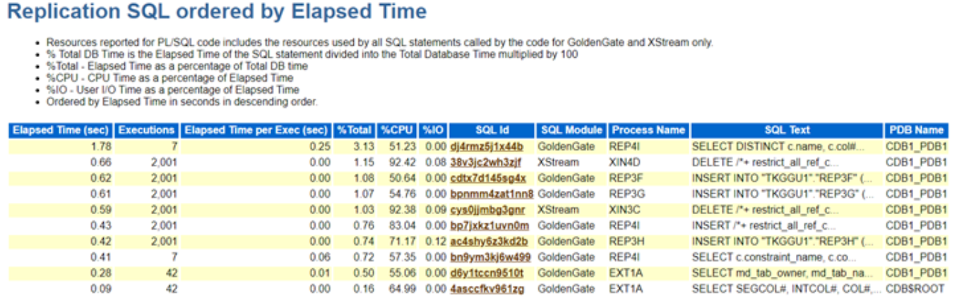
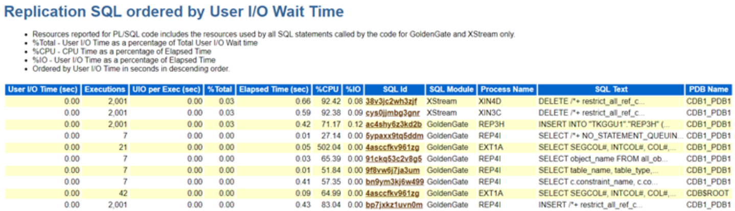
Replication Top SQLs: This highlights the SQL statements executed by various replication processes, organized by key performance metrics such as Elapsed Time, CPU Time, and Execution Count. These sections in the Top SQL report provide a detailed breakdown, allowing administrators to quickly identify the most resource-intensive SQL queries impacting replication performance.

In addition, the replication process name is included for each SQL statement, making it easy to trace which process—whether Extract or Replicat—is responsible for executing the query. This level of granularity helps streamline troubleshooting efforts, as it enables pinpointing of inefficient SQL statements and their impact on replication. The inclusion of these metrics ensures that administrators have the necessary visibility to optimize SQL execution within replication processes, leading to improved overall system performance.

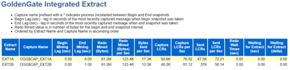
Oracle GoldenGate Extract Performance Metrics : This section explains more in Extract and Capture processes. It provides some really valuable information like ..

  • Lag (in seconds) derived by the time when the most recent LCR was created and received (measured both at the beginning and end)
  • The amount of redo data mined (in bytes).
  • Redo Mined Rate
  • Number of bytes sent by the Capture process to the Extract process since the last time the Extract process attached to the Capture process.
  • Number of LCRs delivered to the Capture from Logminer …. and much more … ….

Oracle GoldenGate Integrated Replicat:

Oracle GoldenGate Replicat: This section presents comprehensive performance statistics for Oracle GoldenGate’s classic, coordinated, and parallel Replicat processes. The SQL operation statistics are aggregated and displayed for each individual Replicat process, providing an overall view of their performance.

Hope It Helped!
Prashant Dixit

Posted in Uncategorized | Tagged: , , , , , , | Leave a Comment »