Tales From A Lazy Fat DBA

Its all about Databases, their performance, troubleshooting & much more …. ¯\_(ツ)_/¯

Posts Tagged ‘performance’

Reading MySQL execution plans without guessing

Posted by FatDBA on July 12, 2026

Every DBA hits this situation eventually. A query that ran in 40 milliseconds last month now takes eleven minutes, nobody deployed anything, and the developer swears the table “isn’t even that big.” The instinct is to add an index and hope. That works often enough to be genuinely dangerous, because it teaches you nothing about why it worked, and the next time the same trick will quietly fail.

The alternative is to read what the optimizer is actually telling you. MySQL is not shy about it. It will hand you its plan, its estimates, and since 8.0.18 .. its real measured execution, if you know how to ask.

Everything below was run on MySQL 8.0.46 against a schema I built specifically to misbehave: 200,000 customers and 1,000,000 orders, with a status column that is dangerously skewed.

CREATE TABLE customers (
  id           INT UNSIGNED NOT NULL AUTO_INCREMENT,
  email        VARCHAR(120) NOT NULL,
  country      CHAR(2)      NOT NULL,
  signup_date  DATE         NOT NULL,
  PRIMARY KEY (id),
  UNIQUE KEY uq_email (email),
  KEY ix_country (country)
) ENGINE=InnoDB;

CREATE TABLE orders (
  id           BIGINT UNSIGNED NOT NULL AUTO_INCREMENT,
  customer_id  INT UNSIGNED    NOT NULL,
  status       VARCHAR(12)     NOT NULL,
  amount       DECIMAL(10,2)   NOT NULL,
  created_at   DATETIME        NOT NULL,
  PRIMARY KEY (id),
  KEY ix_customer (customer_id),
  KEY ix_status (status)
) ENGINE=InnoDB;


-- The skew is the whole point:

status      rows_actual   pct
shipped        980123    98.012
pending         12043     1.204
cancelled        4876     0.488
refunded         2958     0.296

Now comes the main topic of discussion, How the optimizer picks the plan ?

MySQL’s optimizer is cost-based, and the machinery is simpler than people assume. There’s no plan cache learning from history, no adaptive feedback loop. Every compilation is a fresh search over possible strategies, and the cheapest estimated plan wins. Before it costs anything, MySQL rewrites the query. Constants get folded (price > 10 * 5 becomes price > 50). Constants get propagated — if you write WHERE a.id = 42 AND a.id = b.a_id, MySQL infers b.a_id = 42 and pushes that predicate straight into b. Simple views get merged into the outer query. And — this one bites people constantly .. an outer join gets silently converted to an inner join if the WHERE clause rejects NULLs on the inner table. Write LEFT JOIN orders o ... WHERE o.status = 'shipped' and you have written an inner join, whether you meant to or not, because a NULL o.status can never equal 'shipped'.

Then comes range analysis, and this is the part that matters most for the rest of this post. For each usable index, MySQL doesn’t just consult stored statistics. It performs an actual B tree search .. records_in_range() .. physically walking into the index to count how many rows fall inside your predicate’s range. This is real work, touching real pages, at plan time.

Join ordering is a greedy search, not exhaustive. Two conditions govern it: optimizer_search_depth (default 62) and optimizer_prune_level (default 1). For three or four tables MySQL will find something near optimal. For fifteen tables it will find a plan, and that plan may be mediocre. Counterintuitively, if you’re joining that many tables and getting bad plans, lowering optimizer_search_depth to 4 or 8 often produces better plans faster, because you stop the optimizer from burning its budget on a search space it can’t cover anyway.

Costs are computed from tunable constants in mysql.server_cost and mysql.engine_cost …. row_evaluate_cost, io_block_read_cost, and friends. You can change them. You almost definately shouldn’t.

Next lets talk about plan generation and tools we have –> Three tools, three different jobs, and people conflate them constantly.

EXPLAIN gives you the plan as a flat table. It does not run the query. It’s fast, it’s compact, and it’s what you reach for 90% of the time. EXPLAIN FORMAT=JSON gives you the same plan with everything EXPLAIN had to leave out .. the actual cost numbers, which key parts were used, which columns get read, and the exact condition attached to each table. Still doesn’t run the query. When EXPLAIN says something confusing, this is where you go to find out why. EXPLAIN ANALYZE (8.0.18+) actually executes the query and reports what really happened alongside what was predicted. This is the one that ends arguments. It’s also the one you should think twice about before running against production on a DELETE— though for SELECTs it’s just a query that costs you its own runtime.

Same query, all three.

mysql> EXPLAIN SELECT c.email, o.amount FROM customers c
    ->   JOIN orders o ON o.customer_id = c.id
    ->  WHERE o.status = 'refunded' AND c.country = 'JP'\G
*************************** 1. row ***************************
           id: 1
  select_type: SIMPLE
        table: o
         type: ref
possible_keys: ix_customer,ix_status
          key: ix_status
      key_len: 50
          ref: const
         rows: 2958
     filtered: 100.00
        Extra: NULL
*************************** 2. row ***************************
           id: 1
  select_type: SIMPLE
        table: c
         type: eq_ref
possible_keys: PRIMARY,ix_country
          key: PRIMARY
      key_len: 4
          ref: shop.o.customer_id
         rows: 1
     filtered: 5.00
        Extra: Using where


-- JSON format adds the details what were hidden
{
  "query_block": {
    "cost_info": { "query_cost": "3665.19" },
    "nested_loop": [
      { "table": {
          "table_name": "o",
          "access_type": "ref",
          "key": "ix_status",
          "used_key_parts": ["status"],
          "key_length": "50",
          "rows_examined_per_scan": 2958,
          "rows_produced_per_join": 2958,
          "filtered": "100.00",
          "cost_info": { "read_cost": "829.74", "eval_cost": "295.80",
                         "prefix_cost": "1125.54" }
      }},
      { "table": {
          "table_name": "c",
          "access_type": "eq_ref",
          "key": "PRIMARY",
          "key_length": "4",
          "ref": ["shop.o.customer_id"],
          "rows_examined_per_scan": 1,
          "rows_produced_per_join": 147,
          "filtered": "5.00",
          "cost_info": { "prefix_cost": "3665.19" },
          "attached_condition": "(`shop`.`c`.`country` = 'JP')"
      }}
    ]
  }
}

prefix_cost is cumulative … 1125.54 after the first table, 3665.19 after both. rows_produced_per_join: 147 is the estimate flowing out of the join. attached_condition shows you exactly what’s being evaluated where, which is worth the verbosity all by itself. And now comes the truth time 🙂

mysql> EXPLAIN ANALYZE SELECT c.email, o.amount FROM customers c
    ->   JOIN orders o ON o.customer_id = c.id
    ->  WHERE o.status = 'refunded' AND c.country = 'JP'\G

-> Nested loop inner join  (cost=4286 rows=148) (actual time=1.18..37.4 rows=56 loops=1)
    -> Index lookup on o using ix_status (status='refunded')
         (cost=1035 rows=2958) (actual time=0.826..11.5 rows=2958 loops=1)
    -> Filter: (c.country = 'JP')
         (cost=0.999 rows=0.05) (actual time=0.00866..0.00866 rows=0.0189 loops=2958)
        -> Single-row index lookup on c using PRIMARY (id=o.customer_id)
             (cost=0.999 rows=1) (actual time=0.00842..0.00844 rows=1 loops=2958)

Read that inner block carefully, because it’s the single most misread thing in MySQL. rows=0.0189 loops=2958 does not mean MySQL found 0.0189 rows. It means the inner side was executed 2,958 times, and averaged 0.0189 rows per execution. Multiply: 0.0189 × 2958 ≈ 56, which is exactly the final row count. Same for timing … actual time=0.00866 is per loop, not total. The total time for that operation is roughly 0.00866 × 2958 ≈ 25ms. Estimated 148 rows, got 56. That’s a 2.6× overestimate, and I’ll come back to where it came from.

Next, lets check all of the columns and values used in the plan and what exact that means..

id : which SELECT this row belongs to. Same number across rows means same query block, and the order those rows appear in is the join order. Different numbers mean subqueries or unions, and a bigger id executes first.

select_type : SIMPLE for a plain query, PRIMARY for the outer part of one with subqueries, SUBQUERY, DERIVED, UNION, MATERIALIZED. If you see DEPENDENT SUBQUERY, tense up: it means the subquery reruns for every outer row.

table : the table, or a synthetic name like <derived2> for a derived table.

type : The access method. Most important column in the output; full section below.

possible_keys : indexes the optimizer considered. NULL here is diagnostic: it means no index could even theoretically serve this predicate, so before you tune anything, go look at whether the right index exists at all.

key : what it actually chose. When possible_keys lists three indexes and key picks one, the other two lost on cost. That’s a decision you can second-guess.

key_len : bytes of the index actually used. This is the column that catches partial index usage, and people ignore it because the calculation/maths looks like magic, but It isn’t:

  • Each column’s base size (INT = 4, BIGINT = 8)
  • +1 byte if the column is NULLable
  • For variable-length strings, +2 bytes for the length prefix
  • Character columns are counted in bytes, not characters — under utf8mb4 that’s 4 bytes per character

Check it against our real output. status is VARCHAR(12) NOT NULL under utf8mb4: 12 × 4 = 48 octets, no null byte, +2 for the length prefix = 50. And EXPLAIN reports key_len: 50. Exactly. ix_country on CHAR(2) gives 2 × 4 = 8, and yes, key_len: 8.

I built a throwaway table to prove the NULL byte is real …

INT NULL      -> key_len: 5     (4 + 1 null byte)
INT NOT NULL  -> key_len: 4
VARCHAR(10) NULL -> key_len: 43 (10*4 + 1 + 2)

Why care? Because on a composite index (a, b, c), key_len tells you how many of those columns are actually doing work. If key_len only accounts for a, then b and c are dead weight for this query and you’ve been fooling yourself about your index.

ref : what’s being compared against the indexed column. const for a literal, or a column name like shop.o.customer_id when the value comes from an earlier table in the join. This is how you read the data flow of a nested loop.

rows : estimated rows examined for this step. Estimated, and in a join it’s per iteration, not total.

filtered : percentage of those rows expected to survive the WHERE conditions that weren’t handled by the index. This is the column everyone skips and shouldn’t, because rows × filtered / 100 is what actually flows to the next table. In the join above, table c shows rows: 1, filtered: 5.00 … MySQL believes 5% of customers are in Japan. It isn’t 5%. There are eight countries in my data and JP is the rarest at about 2%. That 5.00 is a guess, and it’s precisely why the join estimate came out at 148 instead of 56.

Extra — everything else, and where the real diagnoses live.

Access types, which is best and the worst ??

const : at most one row, matched on a primary key or unique index against a literal. MySQL reads it once during optimization and substitutes it as a constant. You cannot do better.

EXPLAIN SELECT email FROM customers WHERE id = 42;
type: const   key: PRIMARY   key_len: 4   ref: const   rows: 1

eq_ref : one row from this table per row from the previous table, via PK or unique index. This is the ideal for the driven side of a join, and it’s what our join got:

type: eq_ref   key: PRIMARY   key_len: 4   ref: shop.o.customer_id   rows: 1

ref : A non-unique index lookup, may return many rows. Perfectly healthy. Our status='refunded' lookup is ref with rows: 2958.

range : index scan over a bounded range. BETWEEN, >, IN (...), LIKE 'foo%'.

EXPLAIN SELECT id FROM orders WHERE id BETWEEN 100 AND 500;
type: range   key: PRIMARY   key_len: 8   rows: 401   Extra: Using where; Using index

401 estimated, 401 actual. B-tree dives are good at this.

index : full scan of the entire index. Not a lookup. It’s ALL wearing a nicer coat, and it’s only cheap because the index is narrower than the table:

EXPLAIN SELECT COUNT(country) FROM customers;
type: index   key: ix_country   rows: 199488   Extra: Using index

ALL : Is a full table scan. Every row, from disk.

EXPLAIN SELECT * FROM orders WHERE amount > 500;
type: ALL   possible_keys: NULL   key: NULL   rows: 997152   filtered: 33.33

Note: possible_keys: NULL : there’s no index on amount, so this was never even a contest. And note rows: 997152 when the table holds exactly 1,000,000 rows. InnoDB’s row count is itself an estimate, sampled, not counted. Don’t trust it to the digit. A full scan is not automatically a bug, by the way. If you’re reading 98% of the table, a scan genuinely is cheaper than a million index lookups each followed by a random row fetch. The bug is a full scan on a selective predicate.

Now lets read ‘EXTRA’:

Using index : a covering index. Everything the query needs lives in the index; the table itself is never touched. This is the single biggest win available in the Extra column, and it’s easy to engineer. Watch this ..

-- before
EXPLAIN SELECT customer_id, status FROM orders WHERE status='refunded';
type: ref   key: ix_status   rows: 2958   Extra: NULL

ALTER TABLE orders ADD INDEX ix_status_cust (status, customer_id);

-- after
type: ref   key: ix_status_cust   rows: 2958   Extra: Using index

Same rows, same access type, but Extra flipped to Using index and we eliminated 2,958 random primary-key lookups.

Using where : MySQL is filtering rows after fetching them from the storage engine. Not fatal on its own. But Using where sitting next to type: ALL and a low filtered is the classic missing-index signature.

Using index condition : Index Condition Pushdown. Different from Using index, and the names are unhelpfully similar. ICP means the condition is evaluated at the index level so non-matching entries never trigger a row fetch. It’s a real optimization, not a warning.

Using temporary : an internal temp table was built, usually for GROUP BY or DISTINCT. In 8.0 it’s TempTable in memory up to temptable_max_ram (default 1GB), then spills to disk. Small ones are fine. Big ones are why your query fell off a cliff.

Using filesort : the results had to be sorted, because no index provided the required order. “Filesort” does not mean it hit disk; it may well sort entirely in memory within sort_buffer_size. Bad name, causes endless confusion. Still, it’s work you might be able to design away with the right index.

Both at once, which is the combination worth hunting for:

EXPLAIN SELECT c.country, SUM(o.amount) t
  FROM customers c JOIN orders o ON o.customer_id = c.id
 WHERE o.status = 'pending'
 GROUP BY c.country ORDER BY t DESC;

table: o   type: ref   key: ix_status   rows: 22536
Extra: Using temporary; Using filesort

The GROUP BY builds the temp table, and the ORDER BY SUM(o.amount) forces the filesort on top of it .. you cannot index your way out of ordering by an aggregate that doesn’t exist until the group is computed. Sometimes the answer is “this is inherent, accept it.” Knowing which it is, is the job.

Scenario one: the cardinality trap (and where the usual advice is wrong)

Here’s where I have to correct something I’ve written myself in the past.

The standard story goes: MySQL assumes uniform distribution, so on a skewed column it wildly misestimates, and histograms fix it. Let’s test that. Two queries, same column, wildly different selectivity:

-- refunded: 2,958 rows, 0.296% of table
type: ref   key: ix_status   rows: 2958   filtered: 100.00

-- shipped: 980,123 rows, 98% of table
type: ref   key: ix_status   rows: 498576   filtered: 100.00

For refunded, rows: 2958 :: the exact true count. Not close. Exact. So much for uniform-distribution assumptions. This is records_in_range() diving into the B-tree and counting for real. But look at shipped: estimated 498,576, and EXPLAIN ANALYZE reports the truth:

-> Index lookup on orders using ix_status (status='shipped')
   (cost=52812 rows=498576) (actual time=2.35..2136 rows=980123 loops=1)

980,123 actual against 498,576 estimated. A 1.97× underestimate … on the unselective value, not the selective one. The dive samples a bounded number of pages; over a huge range it extrapolates, and extrapolation drifts. So, surely a histogram fixes it?

ANALYZE TABLE orders UPDATE HISTOGRAM ON status WITH 16 BUCKETS;
-- re-run, WITH histogram in place
type: ref   key: ix_status   rows: 498576   filtered: 100.00

Nothing changed. Identical estimate. This is the finding I did not expect, and it’s the most useful thing in this post: when a usable index exists, the index dive wins and the histogram is ignored for the rows estimate.m Histograms feed filtered, not rows. To see them work, take the index away:

-- ix_status dropped
type: ALL   possible_keys: NULL   rows: 997152   filtered: 0.30   Extra: Using where

-> Filter: (orders.status = 'refunded')  (cost=100912 rows=2949)
   (actual time=0.83..251 rows=2958 loops=1)
    -> Table scan on orders  (cost=100912 rows=997152)
       (actual time=0.738..200 rows=1e+6 loops=1)

filtered: 0.30 against a true 0.296%. Estimated 2,949 rows, actual 2,958. The histogram is superb — but only where the optimizer had nothing better.

The practical rule, then, is the opposite of the folklore. Build histograms on columns you are filtering on but have not indexed … typically because they’re low-cardinality and an index would be pointless, but they still need a decent filtered estimate to drive join ordering. Indexing the column and histogramming it is mostly wasted effort. One more trap while we’re in here. Look at the stored histogram:

"buckets": [
  ["base64:type254:Y2FuY2VsbGVk", 0.004594302009347028],
  ["base64:type254:cGVuZGluZw==",  0.01689858210334539],
  ["base64:type254:cmVmdW5kZWQ=",  0.019855833971430835],
  ["base64:type254:c2hpcHBlZA==",  1.0]
],
"histogram-type": "singleton",
"sampling-rate": 0.07373942163752957

Those are cumulative frequencies, not per-value. refunded is not 1.98% of the table … it’s 0.0199 − 0.0169 = 0.0030, i.e. 0.30%. The per-value frequency is the difference between consecutive buckets. I have watched people read that 1.0 on shipped and conclude the histogram is broken. And while we’re looking at bad statistics, check what InnoDB thinks ix_status contains:

INDEX_NAME    COLUMN_NAME    CARDINALITY
ix_status     status         3
ix_customer   customer_id    197646
PRIMARY       id             997152

Cardinality 3. There are four distinct statuses. The default 20 page sample (innodb_stats_persistent_sample_pages) missed one entirely. If you have a low-cardinality column with a rare value that matters, raise that setting for the table and re-analyze … otherwise the optimizer is reasoning about a value it doesn’t know exists.

Scenario two: join order, and why it’s the whole game

Nested-loop joins have a brutal asymmetry: the driving table’s row count becomes the loop count for everything after it. Get it backwards and you multiply your own pain. MySQL got our join right. It drove from orders (2,958 refunded rows) and probed customers by primary key:

-> Nested loop inner join  (cost=4286 rows=148) (actual time=1.18..37.4 rows=56 loops=1)
    -> Index lookup on o using ix_status (status='refunded')
         (cost=1035 rows=2958) (actual ... rows=2958 loops=1)
    -> Filter: (c.country = 'JP')
         (cost=0.999 rows=0.05) (actual ... rows=0.0189 loops=2958)

2,958 loops. 37.4ms. …. Now let’s force the mistake with STRAIGHT_JOIN, which pins join order to the order you wrote:

-> Nested loop inner join  (cost=7692 rows=202) (actual time=1.2..93.1 rows=56 loops=1)
    -> Index lookup on c using ix_country (country='JP')
         (cost=920 rows=4039) (actual ... rows=4039 loops=1)
    -> Filter: (o.status = 'refunded')
         (cost=1.2 rows=0.05) (actual ... rows=0.0139 loops=4039)
        -> Index lookup on o using ix_customer (customer_id=c.id)
             (cost=1.2 rows=4.79) (actual ... rows=5.03 loops=4039)

4,039 loops. 93.1ms. Identical 56 rows out, two and a half times the time. And the inner side is worse than the loop count suggests: each of those 4,039 loops now fetches ~5 orders and throws nearly all of them away (rows=5.03 in, rows=0.0139 surviving the filter). We’re reading roughly 20,000 order rows to keep 56.

The optimizer picked correctly here. It doesn’t always … and when it doesn’t, the reason is almost always upstream: a filtered percentage built on a guess. Recall that filtered: 5.00 on customers. MySQL had no histogram on country, so it fell back to a canned guess, and that guess is what produced the 148-row estimate against 56 actual. On this query the error was harmless. On a five-table join, an error like that at step one compounds through every subsequent step, and that is how you get a plan that’s wrong by four orders of magnitude. While we’re here: filtered: 33.33 on the amount > 500 scan earlier is the same phenomenon in its purest form. That number is not measured. It’s MySQL’s hardcoded 1/3 guess for a range condition on a column it knows nothing about. Any time you see 33.33, 11.11, or 5.00 in filtered, you are looking at a guess, not a statistic.

Selecting and validating indexes

Start with the predicate, not the query text. Equality columns go first in a composite index, then range columns, then columns needed only for ORDER BY or covering. The reason is mechanical: a B tree can only use one range column before the ordering breaks down for everything to its right.

Check key_len to confirm the index is being used as far as you think it is. If your index is (status, customer_id, created_at) and key_len comes back as 50, only status is doing work.

Aim for Using index in Extra where you can. Adding one column to an existing index to make it covering is often a bigger win than adding a whole new index … and it costs you far less on write throughput.

Then validate with EXPLAIN ANALYZE, and compare estimated against actual. A ratio inside about 10× is usually fine. Beyond that, ask why: stale stats (run ANALYZE TABLE), a sample too small to see your rare values (raise innodb_stats_persistent_sample_pages), or a filtered built on a guess (histogram the column … as long as it isn’t already indexed).

Finally, resist the urge to just add the index. Every index is a write tax on every INSERT, UPDATE, and DELETE against that table, forever. Before you create one, check sys.schema_unused_indexes and sys.schema_redundant_indexes … I have never once run those on a mature production system and not found something to drop.

So, in short, summary, EXPLAIN tells you the plan. FORMAT=JSON tells you the costs behind it. EXPLAIN ANALYZE tells you the truth, and the truth is the only one of the three you can act on with confidence. Read rows and filtered together, always, because rows × filtered / 100 is what actually flows downstream. Treat loops as a multiplier, and remember that rows= and actual time= on an inner node are per loop. And when filtered shows you 33.33 or 5.00, recognise it for what it is: MySQL shrugging.

Then go and check whether the optimizer’s guess matched reality. Usually it does. The eleven-second query is where it didn’t.

Hope It Helped!
Prashant Dixit
Posted in Uncategorized | Tagged: , , , | Leave a Comment »

When MySQL OPTIMIZE TABLE made the file bigger instead of smaller and how old_alter_table solved the issue …

Posted by FatDBA on July 2, 2026

Every DBA has had that moment where a command looks simple on paper, but the database decides to teach you a lesson in production-style humility. For me, this happened during a MySQL InnoDB space reclaim activity. The task looked straightforward. We had a few large InnoDB tables where a lot of data had been deleted or moved over time. The logical data inside the table was much smaller than the physical .ibd file sitting on disk. So the goal was simple: rebuild the table, compact the data, and return unused space back to the filesystem.

In MySQL terms, this usually means running —–> OPTIMIZE TABLE XXXX;

The environment was MySQL Community Server 8.0.43. The tables were InnoDB tables, using innodb_file_per_table, which means each table had its own .ibd file on disk. That part is important because if the table is stored in its own file per table tablespace, rebuilding the table can physically shrink the .ibd file and return unused space back to the operating system … At least, that was the expectation. Before starting, we checked the table size from MySQL and from the operating system. For example, one test table, let’s call it appdata.customer_activity_history, had a physical .ibd file that was much larger than the active data inside the table.

The checks were simple and familiar:

SELECT NAME, SPACE_TYPE, ROW_FORMAT, PAGE_SIZE, ROUND(FILE_SIZE/1024/1024/1024,2) AS FILE_SIZE_GB, ROUND(ALLOCATED_SIZE/1024/1024/1024,2) AS ALLOCATED_SIZE_GB, 
STATE FROM information_schema.INNODB_TABLESPACES WHERE NAME = 'appdata/customer_activity_history';

-- And from the OS side:
du -sh /var/lib/mysql/appdata/customer_activity_history.ibd

The table had a clear gap. The .ibd file was large, and based on the data pattern, we expected a rebuild to reclaim a good amount of space. So we ran the usual command —> OPTIMIZE TABLE appdata.customer_activity_history

The command completed, and MySQL returned the familiar InnoDB message … “Table does not support optimize, doing recreate + analyze instead” .. BTW, this message is normal for InnoDB. It simply means MySQL is not doing a classic MyISAM style optimize. For InnoDB, MySQL translates the operation into a table rebuild and analyze style operation.

mysql> OPTIMIZE TABLE appdata.customer_activity_history;

+----------------------------------+----------+----------+-------------------------------------------------------------------+
| Table                            | Op       | Msg_type | Msg_text                                                          |
+----------------------------------+----------+----------+-------------------------------------------------------------------+
| ppdata.customer_activity_history | optimize | note     | Table does not support optimize, doing recreate + analyze instead |
| ppdata.customer_activity_history | optimize | status   | OK                                                                |
+----------------------------------+----------+----------+-------------------------------------------------------------------+

2 rows in set (3 hours 8 min 33.18 sec)

But then came the surprise. When we checked the .ibd file again, the space was not reclaimed as expected. In some cases, the file looked almost the same. In other cases, it actually increased. That is the kind of thing that makes you stop for a minute.

You run a command to reclaim space, wait for a long table rebuild to finish, and then the file gets bigger. Not exactly the kind of result you want to explain with confidence. The first reaction was to question the obvious things. Was the table really using InnoDB? Was innodb_file_per_table enabled? Was the file we checked really the correct .ibd file? Were there long-running transactions? Was there enough free disk space? Was this table partitioned? Were stats outdated? Was the table still holding more active data than expected?

All of those checks were important. Nothing looked wrong from a basic validation point of view. The table was InnoDB. The table had its own .ibd file. The table was accessible. There was enough disk space. The command completed successfully. But the physical reclaim was still not happening the way we expected.

At this point, the issue looked less like a data problem and more like a rebuild method problem. The fix came from changing how MySQL performed the rebuild. Instead of relying on the default optimized ALTER behavior, we forced MySQL to use the older copy style ALTER method by setting this session parameter before running the optimize command …. old_alter_table

Then we ran the optimize again in the same session:

SET old_alter_table=1;
OPTIMIZE TABLE appdata.customer_activity_history;

This small change made the difference … with old_alter_table=1, MySQL does not use the newer optimized ALTER processing method. It falls back to the older temporary table copy method. In simple words, MySQL creates a new copy of the table, copies the active data into it, rebuilds the indexes, and then renames the rebuilt table back into place. That copy style rebuild gave us the clean physical rebuild we were looking for.

After running the command with the session parameter enabled, we checked the .ibd file again and this time, the file size reduced as expected. That was the “okay, now we are getting somewhere” moment.

But one successful table is not enough. A DBA never trusts one clean result when dealing with large tables and filesystem reclaim. So we repeated the same process on a few more large InnoDB tables and for each table, we followed the same careful pattern. We checked the file size before starting. We checked available disk space. We made sure there were no obvious long-running transactions or blockers. We ran SET old_alter_table=1; in the same MySQL session. Then we ran OPTIMIZE TABLE. After it completed, we checked the .ibd file again from the OS level and validated that the table was still accessible.

The important part was not just that the command completed. The important part was that the physical file size actually reduced after the operation. That confirmed the workaround was repeatable. One detail that should not be missed is that old_alter_table is a session-level setting when set this way. It is not something you run once in one window and then assume it applies everywhere forever. If the MySQL session disconnects, or if you open a new MySQL session, you need to run it again before the next OPTIMIZE TABLE. NOTE: This being reverted to old mechanism, now you will see DMLs are blocked and only SELECTS are allowed. Be cautious about it and should perform this task in downtime.

Another important point is disk space. This type of rebuild can temporarily require extra space because MySQL may need space for the rebuilt copy while the operation is running. So even though the final result may be a smaller .ibd file, you still need enough free filesystem space before starting. This is especially important when working with hundreds of GBs or TB-sized tables. This is also not something I would run blindly across many tables in parallel. Large InnoDB rebuilds can be heavy. They can consume I/O, generate temporary space usage, affect replication lag if replication is involved, and introduce metadata locking during parts of the operation. The more controlled approach is to run one table at a time, validate the result, then move to the next one.

The other lesson here is about expectations. OPTIMIZE TABLE sounds like a simple maintenance command, but with InnoDB it is really a table rebuild operation. And with large InnoDB tables, the rebuild method matters. The command can complete successfully from MySQL’s point of view, but that does not always mean the physical reclaim result will match what you expected. In our case, the standard optimize path did not reclaim space correctly and even increased the .ibd file size in some cases. After we added the session command SET old_alter_table=1; immediately before OPTIMIZE TABLE, MySQL used the copy-style rebuild method, and the .ibd file started shrinking as expected. The final version of the approach was simple ..

-- In the session run below param 
SET old_alter_table=1;

-- Now all set to run the optimize command and to avoid the issue
OPTIMIZE TABLE appdata.customer_activity_history;

-- Then validate from the OS:
du -sh /var/lib/mysql/appdata/customer_activity_history.ibd

-- And validate from MySQL:
SELECT
    table_schema,
    table_name,
    ROUND((data_length + index_length)/1024/1024/1024, 2) AS logical_gb,
    table_rows
FROM information_schema.tables
WHERE table_schema = 'appdata'
  AND table_name = 'customer_activity_history';

So if you ever run OPTIMIZE TABLE on a large MySQL InnoDB table and the .ibd file does not shrink, or worse, it grows, do not panic immediately. First, verify the basics. Confirm the storage engine, confirm innodb_file_per_table, check the physical file, check the logical size, and make sure you have enough disk space. It is a small setting, but in this case, it made a big difference.

And yes, sometimes the most useful DBA lessons start with a command doing the exact opposite of what you expected.Then, if the default rebuild path is not giving the expected reclaim, test the session-level copy-style rebuild method carefully

Hope It Helped!
Prashant Dixit

Posted in Uncategorized | Tagged: , , , , | Leave a Comment »

Why oracle’s optimizer has been getting smarter for 15 years and what 26ai version actually adds

Posted by FatDBA on March 31, 2026

Every bad execution plan you’ve ever debugged traces back to the same root cause. The optimizer made a wrong guess about how many rows an operation would return ..and built an entire plan on top of that wrong number.

That number is called cardinality. It’s the estimated row count for each operation in your plan. Get it right and the optimizer picks the right join order, the right join method, the right access path. Get it wrong and you get a nested loops join against a table that returns 500,000 rows when the optimizer thought it was 12. You’ve seen this plan. It hurt.

Oracle has been progressively solving this problem for 15+ years. The story isn’t a single breakthrough ..it’s a series of increasingly smarter mechanisms, each one handling a class of estimation problem that the previous one couldn’t.

Here’s the full honest picture, ending with what 26ai actually adds.

Oracle 10g .. Dynamic Sampling The optimizer noticed when stats were missing or insufficient and sampled the data at parse time to get a rough estimate. Controlled by OPTIMIZER_DYNAMIC_SAMPLING. Blunt instrument, but better than pure guesswork.

Oracle 11g .. Cardinality Feedback The optimizer started comparing its estimates to reality after execution. If it estimated 50 rows and got 50,000, it stored the real number in the SGA and flagged the statement for re-optimization on the next execution. The estimate corrected itself over time. The problem: stored in SGA only — lost on restart, lost when the cursor aged out.

Oracle 12c …The Big Jump Three things landed together:

  • Statistics Feedback (renamed from Cardinality Feedback): same learning mechanism, better persistence
  • Adaptive Plans: the optimizer could now switch join methods mid-execution .. starting with Nested Loops based on its estimate, and switching to Hash Join live if actual rows exceeded the threshold. The final plan was then fixed for subsequent executions
  • SQL Plan Directives: when a misestimate was detected, the optimizer created a persistent directive (stored in SYSAUX, survives restarts) that told future parses: “when you see this predicate pattern, gather dynamic statistics first”. Directives are cross-statement … query’s lesson protects another with the same predicate pattern

Oracle 19c/23ai ..Automation at Scale Automatic SQL Tuning Sets (ASTS), Automatic SPM, and Real-Time SPM turned the individual learning mechanisms into a system-level feedback loop. The database wasn’t just learning from single statements .. it was maintaining plan stability across the entire workload automatically.

Oracle 26ai (23.8 RU) .. The Specific New Additions Two documented, named improvements to cardinality estimation:

  1. Dynamic Statistics for PL/SQL Functions : a new parameter plsql_function_dynamic_stats giving fine-grained control over whether PL/SQL functions called inside SQL can participate in dynamic statistics sampling at parse time. Previously the optimizer treated PL/SQL functions as black boxes with unknowable return cardinality. Now it can sample them.
  2. PL/SQL to SQL Transpiler : when enabled, the optimizer inlines eligible PL/SQL functions directly into SQL at parse time, eliminating the black box entirely. The optimizer can now see and estimate the underlying SQL expression rather than guessing at what a function returns.

Plus the general continued improvement of ML-informed cost models inside the optimizer engine .. real, but not a named switchable feature.

Now let’s see all of this in the plan output where it actually matters and I will do a quick demo — The single most important diagnostic habit in Oracle performance work. The GATHER_PLAN_STATISTICS hint tells the optimizer to track actual row counts during execution, then ALLSTATS LAST in DBMS_XPLAN surfaces them alongside the estimates.

-- Prereqs (run as SYS)
GRANT ADVISOR TO sh;
GRANT ADMINISTER SQL MANAGEMENT OBJECT TO sh;

CONN sh/sh

-- Set output format for readable plans
SET LINESIZE 200
SET PAGESIZE 10000
SET LONG 100000

-- Run the query with stats collection enabled
SELECT /*+ GATHER_PLAN_STATISTICS */
  c.cust_state_province,
  COUNT(*)           AS num_orders,
  SUM(s.amount_sold) AS revenue
FROM   sales     s
JOIN   customers c ON s.cust_id = c.cust_id
WHERE  c.cust_state_province = 'CA'
AND    c.cust_income_level   = 'G: 130,000 - 149,999'
GROUP  BY c.cust_state_province;


SELECT *
FROM TABLE(DBMS_XPLAN.DISPLAY_CURSOR(
  sql_id          => NULL,
  cursor_child_no => 0,
  format          => 'ALLSTATS LAST +COST'
));
```

**Output — before extended statistics exist:**
```
Plan hash value: 3421987654

-------------------------------------------------------------------------------------------
| Id | Operation            | Name      | Starts | E-Rows | A-Rows | Cost  | Buffers |
-------------------------------------------------------------------------------------------
|  0 | SELECT STATEMENT     |           |      1 |        |      1 |  1891 |    1533 |
|  1 |  HASH GROUP BY       |           |      1 |      1 |      1 |  1891 |    1533 |
|* 2 |   HASH JOIN          |           |      1 |     17 |    127 |  1890 |    1533 |  <- E:17, A:127
|* 3 |    TABLE ACCESS FULL | CUSTOMERS |      1 |     17 |    127 |   406 |    1213 |  <- E:17, A:127
|   4|    PARTITION RANGE   |           |      1 |    918K|    918K|  1459 |     320 |
|   5|     TABLE ACCESS FULL| SALES     |     28 |    918K|    918K|  1459 |     320 |
-------------------------------------------------------------------------------------------

Predicate Information:
   2 - access("S"."CUST_ID"="C"."CUST_ID")
   3 - filter("C"."CUST_STATE_PROVINCE"='CA'
          AND "C"."CUST_INCOME_LEVEL"='G: 130,000 - 149,999')

E-Rows: 17. A-Rows: 127. That’s a 7.5x underestimate.

The optimizer assumed cust_state_province = 'CA' and cust_income_level = 'G: 130,000 - 149,999' were independent. They’re not — they’re correlated. California has a disproportionate number of high-income customers in this dataset. The optimizer applied the selectivity of each predicate independently, multiplied them, and got the wrong answer.

This is the classic multi-column predicate correlation problem. The fix is extended statistics.

Lets try to fix it via extended statistics: Extended statistics (column groups) teach the optimizer about correlated columns. One DBMS_STATS call, no schema changes.

-- Create a column group for the two correlated columns
SELECT DBMS_STATS.CREATE_EXTENDED_STATS(
  ownname  => 'SH',
  tabname  => 'CUSTOMERS',
  extension => '(CUST_STATE_PROVINCE, CUST_INCOME_LEVEL)'
) AS col_group_name
FROM DUAL;

-- COL_GROUP_NAME
-- SYS_STUFBF#JKQM8F3GTPA7XDE9  (system-generated name)

-- Now gather stats to populate the column group
EXEC DBMS_STATS.GATHER_TABLE_STATS(
  ownname    => 'SH',
  tabname    => 'CUSTOMERS',
  method_opt => 'FOR ALL COLUMNS SIZE AUTO'
);


---- Lets re runn the same Sql.
SELECT /*+ GATHER_PLAN_STATISTICS */
  c.cust_state_province,
  COUNT(*)           AS num_orders,
  SUM(s.amount_sold) AS revenue
FROM   sales     s
JOIN   customers c ON s.cust_id = c.cust_id
WHERE  c.cust_state_province = 'CA'
AND    c.cust_income_level   = 'G: 130,000 - 149,999'
GROUP  BY c.cust_state_province;

SELECT *
FROM TABLE(DBMS_XPLAN.DISPLAY_CURSOR(
  sql_id          => NULL,
  cursor_child_no => 0,
  format          => 'ALLSTATS LAST +COST'
));


After extended statistics:
Plan hash value: 3421987654

-------------------------------------------------------------------------------------------
| Id | Operation            | Name      | Starts | E-Rows | A-Rows | Cost  | Buffers |
-------------------------------------------------------------------------------------------
|  0 | SELECT STATEMENT     |           |      1 |        |      1 |  1891 |    1533 |
|  1 |  HASH GROUP BY       |           |      1 |      1 |      1 |  1891 |    1533 |
|* 2 |   HASH JOIN          |           |      1 |    124 |    127 |  1890 |    1533 |  <- E:124, A:127
|* 3 |    TABLE ACCESS FULL | CUSTOMERS |      1 |    124 |    127 |   406 |    1213 |  <- Near perfect
|   4|    PARTITION RANGE   |           |      1 |    918K|    918K|  1459 |     320 |
|   5|     TABLE ACCESS FULL| SALES     |     28 |    918K|    918K|  1459 |     320 |
-------------------------------------------------------------------------------------------

E-Rows went from 17 to 124. Actual is 127. That’s less than 3% off.

Same plan hash .. same shape. But now the cost model is working from accurate numbers. In a more complex query, this difference in estimated rows would change join order, join method, and index decisions.

nEXT, Lets see SQL Plan directives and see watching optimizer learn.

When the optimizer detects a cardinality misestimate during execution, it creates a SQL Plan Directive — a persistent instruction stored in SYSAUX telling future parses to gather dynamic statistics for this predicate pattern. You can watch this happen.

First, drop the extended stats so the misestimate recurs:

-- Reset: drop the column group
EXEC DBMS_STATS.DELETE_EXTENDED_STATS(
  ownname   => 'SH',
  tabname   => 'CUSTOMERS',
  extension => '(CUST_STATE_PROVINCE, CUST_INCOME_LEVEL)'
);

EXEC DBMS_STATS.GATHER_TABLE_STATS('SH', 'CUSTOMERS');

-- lets fliush the SP and re-run.

-- As SYS (flush shared pool in test environment only)
ALTER SYSTEM FLUSH SHARED_POOL;

CONN sh/sh

-- Run with stats collection
SELECT /*+ GATHER_PLAN_STATISTICS */
  c.cust_state_province,
  COUNT(*), SUM(s.amount_sold)
FROM   sales s
JOIN   customers c ON s.cust_id = c.cust_id
WHERE  c.cust_state_province = 'CA'
AND    c.cust_income_level   = 'G: 130,000 - 149,999'
GROUP  BY c.cust_state_province;


-- Lets see if the directive was crwated. 

-- Check for new SQL Plan Directives on CUSTOMERS
SELECT d.directive_id,
       d.type,
       d.state,
       d.auto_drop,
       d.created,
       o.object_name,
       o.subobject_name  AS column_name
FROM   dba_sql_plan_directives     d
JOIN   dba_sql_plan_dir_objects    o
       ON d.directive_id = o.directive_id
WHERE  o.object_name = 'CUSTOMERS'
ORDER  BY d.created DESC;


Output — directive created after the misestimate:

DIRECTIVE_ID  TYPE             STATE   AUTO_DROP CREATED              OBJECT  COLUMN_NAME
------------  ---------------  ------  --------- -------------------  ------  -------------------
8273641920    DYNAMIC_SAMPLING USABLE  YES        2026-03-29 14:33:12 CUSTOMERS CUST_STATE_PROVINCE
8273641920    DYNAMIC_SAMPLING USABLE  YES        2026-03-29 14:33:12 CUSTOMERS CUST_INCOME_LEVEL

The optimizer created a directive covering both columns … it noticed the multi-column predicate correlation caused a misestimate and now knows to sample dynamically next time it sees this pattern. Run the query a second time:

SELECT /*+ GATHER_PLAN_STATISTICS */
  c.cust_state_province,
  COUNT(*), SUM(s.amount_sold)
FROM   sales s
JOIN   customers c ON s.cust_id = c.cust_id
WHERE  c.cust_state_province = 'CA'
AND    c.cust_income_level   = 'G: 130,000 - 149,999'
GROUP  BY c.cust_state_province;

SELECT *
FROM TABLE(DBMS_XPLAN.DISPLAY_CURSOR(
  format => 'ALLSTATS LAST +NOTE'
));


At the bottom of the plan output:
Note
-----
   - dynamic statistics used: dynamic sampling (level=2)
   - 1 Sql Plan Directive used for this statement

The optimizer is now dynamically sampling at parse time because the directive told it to. The cardinality estimate will be much closer to reality on this execution.

Now new in 26ai ..The SQL aanalysis report .. This is the part that’s genuinely new in 26ai. Previously you had to know to look at E-Rows vs A-Rows yourself. The SQL Analysis Report .. surfaced directly in DBMS_XPLAN.DISPLAY_CURSOR output …flags these problems inline without you having to hunt for them.

-- The standard DISPLAY_CURSOR call — no extra parameters needed
-- SQL Analysis Report appears automatically in 26ai when issues exist

SELECT *
FROM TABLE(DBMS_XPLAN.DISPLAY_CURSOR(
  sql_id          => NULL,
  cursor_child_no => 0,
  format          => 'ALLSTATS LAST +COST'
));


In Oracle 26ai, after the standard execution plan output, you now see:

SQL Analysis Report (identified by operation id/Query Block Name/Object Alias):
--------------------------------------------------------------------------------
3 - SEL$1 / "C"@"SEL$1"
  - The following columns have predicates which prevent their use as keys
    in an index range scan. Consider rewriting the predicates or creating
    column group statistics.
    "CUST_STATE_PROVINCE", "CUST_INCOME_LEVEL"

The optimizer is telling you directly: these two columns in combination are causing an estimation problem, and column group statistics would fix it. You no longer have to derive this by comparing E-Rows and A-Rows yourself. It’s surfaced automatically in the plan output.

That’s a real DBA quality-of-life improvement. The diagnosis that used to take 10 minutes of plan reading is now one line in your standard plan output.

Okay next is Dynamic Stats for PL/SQL Functions …. This is the specific new documented feature in 26ai (RU 23.8). Consider a query that filters through a PL/SQL function:

-- A function the optimizer previously couldn't estimate
CREATE OR REPLACE FUNCTION sh.get_high_value_threshold
RETURN NUMBER DETERMINISTIC IS
BEGIN
  RETURN 1000;
END;
/

-- Query using the function in a predicate
SELECT /*+ GATHER_PLAN_STATISTICS */
  COUNT(*),
  SUM(amount_sold)
FROM   sh.sales
WHERE  amount_sold > sh.get_high_value_threshold();


Before 26ai (or with `plsql_function_dynamic_stats = 'OFF'`):

The optimizer treats `get_high_value_threshold()` as a black box. It has no idea what value the function returns, 
so it can't estimate selectivity. It either guesses based on defaults or uses a very conservative estimate.

| Id | Operation            | Name  | E-Rows | A-Rows |
|  0 | SELECT STATEMENT     |       |        |      1 |
|  1 |  SORT AGGREGATE      |       |      1 |      1 |
|* 2 |   PARTITION RANGE ALL|       |   9188 |  12116 |  <- Rough guess
|*  3|    TABLE ACCESS FULL | SALES |   9188 |  12116 |

In 26ai with plsql_function_dynamic_stats = 'ON':

-- Enable dynamic stats for PL/SQL functions (session level)
ALTER SESSION SET plsql_function_dynamic_stats = 'ON';

-- Rerun
SELECT /*+ GATHER_PLAN_STATISTICS */
  COUNT(*),
  SUM(amount_sold)
FROM   sh.sales
WHERE  amount_sold > sh.get_high_value_threshold();

SELECT *
FROM TABLE(DBMS_XPLAN.DISPLAY_CURSOR(
  format => 'ALLSTATS LAST +NOTE'
));


| Id | Operation            | Name  | E-Rows | A-Rows |
|  0 | SELECT STATEMENT     |       |        |      1 |
|  1 |  SORT AGGREGATE      |       |      1 |      1 |
|* 2 |   PARTITION RANGE ALL|       |  12203 |  12116 |  <- Near accurate
|*  3|    TABLE ACCESS FULL | SALES |  12203 |  12116 |

Note
-----
   - dynamic statistics used: dynamic sampling (level=2)
   - PL/SQL function sampled for dynamic statistics

The optimizer called the function during dynamic statistics gathering at parse time, got the actual return value (1000), and used it to estimate selectivity accurately. E-Rows 12,203 vs A-Rows 12,116 — less than 1% off.

You can also control this at the object level, which is the right approach in production .. turn it on only for specific functions you trust:

-- Prefer object-level control in production
-- Allow dynamic stats for a specific function
EXEC DBMS_STATS.SET_FUNCTION_PREFS(
  ownname   => 'SH',
  funcname  => 'GET_HIGH_VALUE_THRESHOLD',
  pref_name => 'PLSQL_FUNCTION_DYNAMIC_STATS',
  pref_value => 'ON'
);

-- Check current settings
SELECT function_name, preference_name, preference_value
FROM   all_stat_extensions
WHERE  object_type = 'FUNCTION'
AND    owner = 'SH';

So, in short, Oracle’s optimizer hasn’t made one big leap … it’s made fifteen years of deliberate, incremental improvements, each one handling a class of cardinality problem the previous release couldn’t.

What 26ai specifically adds isn’t magic. It’s two concrete, named, documented improvements … dynamic statistics for PL/SQL functions, and the SQL Analysis Report surfacing optimizer advice inline .. plus the PL/SQL transpiler removing the problem class entirely for eligible functions. These are real. They’re testable. They’re in the docs.

The underlying ML enhanced cost modelling is also real, but it’s an evolutionary improvement without a named switch … Oracle’s engineering continues to get better at estimating costs, particularly for complex workloads, vector queries, and correlated predicates. That’s not hype. It’s just not a single feature you can point to in the docs either.

Know your E-Rows vs A-Rows. Know your SQL Plan Directives. Know your extended statistics. And in 26ai, let the SQL Analysis Report do the first pass for you.

Hope It Helped!
Prashant Dixit

Posted in Uncategorized | Tagged: , , , , , , , | Leave a Comment »

Cleaning Up MySQL Replication Checks With a Bit of Bash

Posted by FatDBA on January 29, 2026

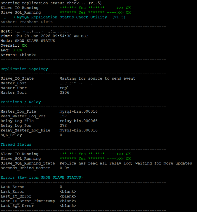
Checking MySQL replication is one of those things DBAs do on autopilot. Log in, open the MySQL client, run SHOW SLAVE STATUS\G or SHOW REPLICA STATUS\G, scroll, scan for Yes, check lag, repeat. It works, but it is noisy, raw, and easy to misread when you are tired or troubleshooting multiple servers.

In some free time, I played around with shell scripting to clean this up. The goal was not to replace MySQL, but to wrap the same information into something that answers the real question faster: is replication healthy or not, and how bad is it if it is not.

The script runs with strict shell settings so failures are never hidden. It connects using a MySQL login path first and falls back to a secure defaults file, which keeps credentials out of the script. If MySQL cannot be reached or authentication fails, the script stops immediately and shows the real error instead of pretending replication is broken.

Because environments are rarely consistent, the script automatically detects whether the server supports SHOW REPLICA STATUS or still uses SHOW SLAVE STATUS. It figures this out by checking for known fields and then sticks to the correct command, which makes it usable across old and new MySQL versions without edits.

Once the raw replication output is captured, the script parses individual fields directly from the \G output using awk. It handles both old and new field names, so Source_Host and Master_Host are treated the same. The same approach is used for thread states, binlog positions, relay logs, delay, and error fields. If replication is not configured and MySQL returns an empty result, the script fails clearly instead of silently succeeding.

From there, it starts behaving more like a DBA than a SQL dump. IO and SQL threads are evaluated and clearly marked as OK, PROBLEM, or UNKNOWN. Replication lag is converted from seconds into minutes and evaluated against simple thresholds so you immediately know whether it is harmless or serious. If any SQL or IO errors exist, replication is considered critical even if threads appear to be running.

One thing I was very deliberate about is that the script always prints the full report, even when replication is stopped or broken. When things go wrong, you still see topology details, binlog and relay positions, thread states, and error messages in one place. Nothing is hidden when you need it the most.

The output is structured like a quick operational report, with hostname, timestamp, replication mode, overall health, lag, and error presence shown at the top. Color highlighting is used only in interactive sessions, so the script remains safe for logging and automation.

Finally, the script exits with meaningful return codes. A clean replication state exits successfully, warning conditions return a different code, and critical failures return a hard error. This makes it easy to plug into cron jobs or monitoring without parsing text output.

This started as a small free-time experiment, but it turned into something I actually use. Shell scripting may not be glamorous, but for DBAs it is one of the fastest ways to remove friction from daily work. If you find yourself running the same replication commands again and again, that is usually a sign that a small script can make life easier.

#!/usr/bin/env bash
set -euo pipefail

# -------------------------------------------------------------------
# Author : Prashant Dixit
# Version: 1.5 (always print full report + cleaner header formatting)
# Notes  : Shows full sections even when replication is stopped / broken.
# -------------------------------------------------------------------

MYSQL_BIN="${MYSQL_BIN:-/usr/bin/mysql}"

MYSQL_LOGIN_PATH="${MYSQL_LOGIN_PATH:-testadmin_local}"

MYSQL_CNF="${MYSQL_CNF:-/root/.my-shutdown.cnf}"

if [[ -t 1 ]]; then
  RED=$'\033[0;31m'
  GREEN=$'\033[0;32m'
  YELLOW=$'\033[0;33m'
  BLUE=$'\033[0;34m'
  CYAN=$'\033[0;36m'
  BOLD=$'\033[1m'
  DIM=$'\033[2m'
  RESET=$'\033[0m'
else
  RED=""; GREEN=""; YELLOW=""; BLUE=""; CYAN=""; BOLD=""; DIM=""; RESET=""
fi

hr()  { printf "%s\n" "${DIM}----------------------------------------------------------------------${RESET}"; }
hdr() { printf "%s\n" "${BOLD}${CYAN}$*${RESET}"; }
die() { echo "${RED}ERROR:${RESET} $*"; exit 2; }

mysql_run() {
  # Try login-path first, fallback to defaults-file
  local q="$1" out rc
  out="$("$MYSQL_BIN" --login-path="$MYSQL_LOGIN_PATH" -e "$q" 2>&1)" && { echo "$out"; return 0; }
  rc=$?

  if [[ -r "$MYSQL_CNF" ]]; then
    out="$("$MYSQL_BIN" --defaults-file="$MYSQL_CNF" -e "$q" 2>&1)" && { echo "$out"; return 0; }
    rc=$?
    echo "$out"
    return $rc
  fi

  echo "$out"
  return $rc
}

detect_status_cmd() {
  # If SHOW REPLICA STATUS works, use it; else fallback to SLAVE
  if mysql_run "SHOW REPLICA STATUS\\G" | grep -qE '^[[:space:]]*(Replica_IO_State|Source_Host):'; then
    echo "SHOW REPLICA STATUS\\G"
  else
    echo "SHOW SLAVE STATUS\\G"
  fi
}

STATUS_CMD="$(detect_status_cmd)"


STATUS_RAW="$(mysql_run "$STATUS_CMD" 2>&1 || true)"

if echo "$STATUS_RAW" | grep -qiE "^(ERROR|mysql:)|Access denied|unknown option|Can't connect|Can't connect to local MySQL server|ERROR [0-9]+"; then
  echo "$STATUS_RAW"
  exit 2
fi


if [[ -z "${STATUS_RAW//[[:space:]]/}" ]]; then
  die "No replica/slave status returned. Is this server configured as a replica?"
fi

get_field() {
  local key="$1"
  echo "$STATUS_RAW" |
    awk -F': ' -v k="$key" '
      {
        gsub(/^[ \t]+|[ \t]+$/, "", $1)
        if ($1 == k) {print $2; found=1; exit}
      }
      END {if (!found) print ""}'
}

Slave_IO_State="$(get_field "Replica_IO_State")"; [[ -n "$Slave_IO_State" ]] || Slave_IO_State="$(get_field "Slave_IO_State")"

Master_Host="$(get_field "Source_Host")"; [[ -n "$Master_Host" ]] || Master_Host="$(get_field "Master_Host")"
Master_User="$(get_field "Source_User")"; [[ -n "$Master_User" ]] || Master_User="$(get_field "Master_User")"
Master_Port="$(get_field "Source_Port")"; [[ -n "$Master_Port" ]] || Master_Port="$(get_field "Master_Port")"

Master_Log_File="$(get_field "Source_Log_File")"; [[ -n "$Master_Log_File" ]] || Master_Log_File="$(get_field "Master_Log_File")"
Read_Master_Log_Pos="$(get_field "Read_Source_Log_Pos")"; [[ -n "$Read_Master_Log_Pos" ]] || Read_Master_Log_Pos="$(get_field "Read_Master_Log_Pos")"

Relay_Log_File="$(get_field "Relay_Log_File")"
Relay_Log_Pos="$(get_field "Relay_Log_Pos")"

Relay_Master_Log_File="$(get_field "Relay_Source_Log_File")"
[[ -n "$Relay_Master_Log_File" ]] || Relay_Master_Log_File="$(get_field "Relay_Master_Log_File")"

SQL_Delay="$(get_field "SQL_Delay")"

Slave_IO_Running="$(get_field "Replica_IO_Running")"; [[ -n "$Slave_IO_Running" ]] || Slave_IO_Running="$(get_field "Slave_IO_Running")"
Slave_SQL_Running="$(get_field "Replica_SQL_Running")"; [[ -n "$Slave_SQL_Running" ]] || Slave_SQL_Running="$(get_field "Slave_SQL_Running")"

Slave_SQL_Running_State="$(get_field "Replica_SQL_Running_State")"
[[ -n "$Slave_SQL_Running_State" ]] || Slave_SQL_Running_State="$(get_field "Slave_SQL_Running_State")"

Seconds_Behind_Master="$(get_field "Seconds_Behind_Source")"
[[ -n "$Seconds_Behind_Master" ]] || Seconds_Behind_Master="$(get_field "Seconds_Behind_Master")"

Last_Errno="$(get_field "Last_Errno")"
Last_Error="$(get_field "Last_Error")"

Last_IO_Error="$(get_field "Last_IO_Error")"
Last_IO_Error_Timestamp="$(get_field "Last_IO_Error_Timestamp")"

Last_SQL_Error="$(get_field "Last_SQL_Error")"

fmt_kv() {
  local k="$1" v="${2:-}"
  [[ -n "${v// /}" ]] || v="<blank>"
  printf "%-24s %s\n" "$k" "$v"
}

emph_status() {
  local label="$1"
  local value="${2:-}"
  local norm="${value,,}"

  [[ -n "${value// /}" ]] || value="<blank>"

  if [[ "$norm" == "yes" ]]; then
    printf "%-24s %s\n" "$label" "${GREEN}******* ${value} ******* ---->>> OK${RESET}"
    return 0
  elif [[ "$norm" == "no" ]]; then
    printf "%-24s %s\n" "$label" "${RED}******* ${value} ******* ---->>> PROBLEM${RESET}"
    return 2
  else
    printf "%-24s %s\n" "$label" "${YELLOW}******* ${value} ******* ---->>> UNKNOWN${RESET}"
    return 1
  fi
}

sec_to_min() {
  local s="${1:-}"
  [[ "$s" =~ ^[0-9]+$ ]] || { echo "<blank>"; return; }

  if (( s < 600 )); then
    awk -v sec="$s" 'BEGIN { printf "%.1fm", sec/60 }'
  else
    awk -v sec="$s" 'BEGIN { printf "%dm", int(sec/60) }'
  fi
}


overall="OK"
overall_color="$GREEN"

io_rc=0; sql_rc=0
emph_status "Slave_IO_Running" "${Slave_IO_Running:-}"; io_rc=$?
emph_status "Slave_SQL_Running" "${Slave_SQL_Running:-}"; sql_rc=$?

if [[ $io_rc -eq 2 || $sql_rc -eq 2 ]]; then
  overall="CRITICAL"; overall_color="$RED"
elif [[ $io_rc -eq 1 || $sql_rc -eq 1 ]]; then
  overall="WARNING"; overall_color="$YELLOW"
fi

lag_hint="<blank>"
if [[ -n "${Seconds_Behind_Master// /}" ]] && [[ "${Seconds_Behind_Master}" =~ ^[0-9]+$ ]]; then
  lag_min="$(sec_to_min "$Seconds_Behind_Master")"
  if (( Seconds_Behind_Master == 0 )); then
    lag_hint="${GREEN}${lag_min}${RESET}"
  elif (( Seconds_Behind_Master <= 30 )); then
    lag_hint="${YELLOW}${lag_min}${RESET}"
    [[ "$overall" == "OK" ]] && overall="WARNING" && overall_color="$YELLOW"
  else
    lag_hint="${RED}${lag_min}${RESET}"
    overall="CRITICAL"; overall_color="$RED"
  fi
fi

err_hint="<blank>"
if [[ -n "${Last_SQL_Error// /}${Last_IO_Error// /}${Last_Error// /}" ]]; then
  err_hint="${RED}Errors present${RESET}"
  overall="CRITICAL"; overall_color="$RED"
fi

clear 2>/dev/null || true

hdr "MySQL Replication Status Check Utility  ${DIM}(v1.5)${RESET}"
echo "${DIM}Author: Prashant Dixit${RESET}"
hr
printf "%s %s\n" "${BOLD}Host:${RESET}" "$(hostname -f)"
printf "%s %s\n" "${BOLD}Time:${RESET}" "$(date)"
printf "%s %s\n" "${BOLD}Mode:${RESET}" "${STATUS_CMD%%\\G}"
printf "%s %s  %s  %s\n" "${BOLD}Overall:${RESET}" "${overall_color}${BOLD}${overall}${RESET}" "${BOLD}Lag:${RESET} ${lag_hint}" "${err_hint}"
hr
echo

hdr "Replication Topology"
hr
fmt_kv "Slave_IO_State" "${Slave_IO_State:-}"
fmt_kv "Master_Host" "${Master_Host:-}"
fmt_kv "Master_User" "${Master_User:-}"
fmt_kv "Master_Port" "${Master_Port:-}"
echo

hdr "Positions / Relay"
hr
fmt_kv "Master_Log_File" "${Master_Log_File:-}"
fmt_kv "Read_Master_Log_Pos" "${Read_Master_Log_Pos:-}"
fmt_kv "Relay_Log_File" "${Relay_Log_File:-}"
fmt_kv "Relay_Log_Pos" "${Relay_Log_Pos:-}"
fmt_kv "Relay_Master_Log_File" "${Relay_Master_Log_File:-}"
fmt_kv "SQL_Delay" "${SQL_Delay:-}"
echo

hdr "Thread Status"
hr
emph_status "Slave_IO_Running" "${Slave_IO_Running:-}"
emph_status "Slave_SQL_Running" "${Slave_SQL_Running:-}"
fmt_kv "Slave_SQL_Running_State" "${Slave_SQL_Running_State:-}"
fmt_kv "Seconds_Behind_Master" "$(sec_to_min "${Seconds_Behind_Master:-}")"
echo

hdr "Errors"
hr
fmt_kv "Last_Errno" "${Last_Errno:-}"
fmt_kv "Last_Error" "${Last_Error:-}"
fmt_kv "Last_IO_Error" "${Last_IO_Error:-}"
fmt_kv "Last_IO_Error_Timestamp" "${Last_IO_Error_Timestamp:-}"
fmt_kv "Last_SQL_Error" "${Last_SQL_Error:-}"
hr
echo

if [[ "$overall" == "OK" ]]; then
  exit 0
elif [[ "$overall" == "WARNING" ]]; then
  exit 1
else
  exit 2
fi

Hope It Helped!
Prashant Dixit

Posted in Uncategorized | Tagged: , , , , , , , | Leave a Comment »

When Linux Swaps Away My Sleep – MySQL, RHEL8, and the Curious Case of High Swap Usage

Posted by FatDBA on December 12, 2025

I remember an old instance where I’d got an alert that one of production MySQL servers had suddenly gone sluggish after moved to RHEL 8 from RHEL7. On checking, I found something odd … the system was consuming swap heavily, even though there was plenty of physical memory free.

Someone who did the first time deployment years before, left THP as enabled and with default swapiness … but this setting that had worked perfectly for years on RHEL 7, but now, after the upgrade to RHEL 8.10, the behavior was completely different.

This post is about how that small OS level change turned into a real performance headache, and what we found after some deep digging.

The server in question was a MySQL 8.0.43 instance running on a VMware VM with 16 CPUs and 64 GB RAM. When the issue began, users complained that the database was freezing randomly, and monitoring tools were throwing high load average and slow query alerts.

Let’s take a quick look at the environment … It was a pretty decent VM, nothing under sized.

$ cat /etc/redhat-release
Red Hat Enterprise Linux release 8.10 (Ootpa)

$ uname -r
4.18.0-553.82.1.el8_10.x86_64

$ uptime
11:20:24 up 3 days, 10:57,  2 users,  load average: 4.34, 3.15, 3.63

$ grep ^CPU\(s\) sos_commands/processor/lscpu
CPU(s): 16

When I pulled the SAR data for that morning, the pattern was clear ..There were long stretches on CPU where %iowait spiked above 20-25%, and load averages crossed 400+ during peak time! The 09:50 slot looked particularly suspicious .. load average jumped to 464 and remained high for several minutes.

09:00:01 %usr=26.08  %iowait=22.78  %idle=46.67
09:40:01 %usr=29.04  %iowait=24.43  %idle=40.11
09:50:01 %usr=7.55   %iowait=10.07  %idle=80.26
10:00:01 %usr=38.53  %iowait=19.54  %idle=35.32

Here’s what the memory and swap stats looked like:

# Memory Utilization
%memused ≈ 99.3%
Free memory ≈ 400 MB (on a 64 GB box)
Swap usage ≈ 85% average, hit 100% at 09:50 AM

That was confusing.. MySQL was not leaking memory, and there was still >10 GB available for cache and buffers. The system was clearly pushing pages to swap even though it didn’t need to. That was the turning point in the investigation.

At the same time, the reporting agent started reporting MySQL timeouts:

 09:44:09 [mysql] read tcp xxx.xx.xx.xx:xxx->xxx.xxx.xx.xx:xxxx: i/o timeout
 09:44:14 [mysql] read tcp xx.xx.xx.xxxx:xxx->xx.xx.xx.xx.xx:xxx: i/o timeout

And the system kernel logs showed the familiar horror lines for every DBA .. MySQL threads were being stalled by the OS. This aligned perfectly with the time when swap usage peaked.

 09:45:34 kernel: INFO: task mysqld:5352 blocked for more than 120 seconds.
 09:45:34 kernel: INFO: task ib_pg_flush_co:9435 blocked for more than 120 seconds.
 09:45:34 kernel: INFO: task connection:10137 blocked for more than 120 seconds.

I double-checked the swappiness configuration:

$ cat /proc/sys/vm/swappiness
1

So theoretically, swap usage should have been minimal. But the system was still paging aggressively. Then I checked the cgroup configuration (a trick I learned from a Red Hat note) .. And there it was more than 115 cgroups still using the default value of 60! … In RHEL 8, memory management moved more toward cgroup v2, which isolates memory parameters by control group.

So even if /proc/sys/vm/swappiness is set to 1, processes inside those cgroups can still follow their own default value (60) and this explained why the system was behaving like swappiness=60 even though the global value was 1.

$ find /sys/fs/cgroup/memory/ -name *swappiness -exec cat {} \; | uniq -c
      1 1
    115 60

In RHEL 8, memory management moved more toward cgroup v2, which isolates memory parameters by control group. So even if /proc/sys/vm/swappiness is set to 1, processes inside those cgroups can still follow their own default value (60). This explained why the system was behaving like swappiness=60 even though the global value was 1.

Once the root cause was identified, the fix was straightforward — Enforced global swapiness across CGroups

Add this to /etc/sysctl.conf:

vm.force_cgroup_v2_swappiness = 1

Then reload:
sysctl -p

This forces the kernel to apply the global swappiness value to all cgroups, ensuring consistent behavior. Next, we handled THP that is always expected to cause intermittent fragmentation and stalls in memory intensive workloads like MySQL, Oracle, PostgreSQL and even in non RDBMSs like Cassandra etc., we disabled the transparent huge pages and rebooted the host.

In short what happened and was the root cause.

  • RHEL8 introduced a change in how swappiness interacts with cgroups.
  • The old /proc/sys/vm/swappiness setting no longer applies universally.
  • Unless explicitly forced, MySQL’s cgroup keeps the default swappiness (60).
  • Combined with THP and background I/O, this created severe page cache churn.

So the OS upgrade, not MySQL, was the real root cause.

Note: https://access.redhat.com/solutions/6785021

Hope It Helped!
Prashant Dixit

Posted in Uncategorized | Tagged: , , , , , , , | Leave a Comment »

From Painful Manual LOB Shrink to Automatic SecureFiles Shrink

Posted by FatDBA on November 15, 2025

I’ve been working with LOBs for years now, and trust me, shrinking them has always been a headache. Anyone who has ever tried ALTER TABLE … SHRINK SPACE on a big SecureFiles LOB knows the pain … blocking sessions, unexpected waits, and sometimes that lovely ORA-1555 popping up at the worst time. Every DBA eventually gets into that situation where a LOB segment is 200 GB on disk but only 10 GB of real data remains. You delete rows… but the space never comes back unless you manually shrink it, which itself can cause more issues.

With the introduction of Automatic SecureFiles Shrink, Oracle really made a DBA’s life easier. This feature, which first came out in 23ai, quietly frees up unused LOB space in the background without disrupting your workload. I wanted to see how it behaves in a real scenario, so I set up a small lab and tested it out. Here’s the whole experiment, raw and simple.

Lets do a demo and understand how this new feature works … I spun up a fresh PDB and made a small tablespace just for this test. Nothing fancy.

CREATE TABLESPACE lobts
  DATAFILE '/u02/oradata/LOBTS01.dbf'
  SIZE 1G AUTOEXTEND ON NEXT 256M;

Tablespace created.


-- Table with a securefile LOB based column.
CREATE TABLE tst_securefile_lob
(
    id NUMBER,
    lob_data CLOB
)
LOB (lob_data) STORE AS SECUREFILE (
    TABLESPACE lobts
    CACHE
);

Table created.


SELECT table_name, column_name, securefile
FROM   user_lobs
WHERE  table_name='TST_SECUREFILE_LOB';

TABLE_NAME           COLUMN_NAME   SECUREFILE
-------------------  ------------  ----------
TST_SECUREFILE_LOB   LOB_DATA      YES


Next, I inserted a good amount of junk data around 10,000 rows of random CLOB strings. I wanted the LOB segment to be big enough to see clear differences after shrink.

BEGIN
  FOR r IN 1 .. 10 LOOP
    INSERT INTO tst_securefile_lob (id, lob_data)
    SELECT r*100000 + level,
           TO_CLOB(DBMS_RANDOM.STRING('x', 32767))
    FROM dual
    CONNECT BY level <= 1000;
    COMMIT;
  END LOOP;
END;
/

PL/SQL procedure successfully completed.


SELECT COUNT(*) FROM tst_securefile_lob;

  COUNT(*)
----------
     10000


SELECT ul.segment_name,
       us.blocks,
       ROUND(us.bytes/1024/1024,2) AS mb
FROM   user_lobs ul
JOIN   user_segments us
  ON us.segment_name = ul.segment_name
WHERE  ul.table_name = 'TST_SECUREFILE_LOB';

SEGMENT_NAME               BLOCKS     MB
------------------------   --------   --------
SYS_LOB0001234567C00002$     131072     1024.00


-- After stats and a quick check in USER_SEGMENTS, the LOB segment was showing a nice chunky size. 
-- Then I deleted almost everything
-- Now the table will have very few rows left, but the LOB segment was still the same size. As usual.
DELETE FROM tst_securefile_lob
WHERE id < 900000;
COMMIT;

9990 rows deleted. 
Commit complete.


-- Checking LOB Internal Usage (Before Auto Shrink)
EXEC show_securefile_space(USER, 'SYS_LOB0001234567C00002$');
Segment blocks      = 131072  bytes=1073741824
Used blocks         =  10240  bytes=83886080
Expired blocks      = 110592  bytes=905969664
Unexpired blocks    =  10240  bytes=83886080
-- This clearly shows almost the entire segment is expired/free but not reclaimed.


-- Checking Auto Shrink Statistics (Before Enabling)
SELECT name, value
FROM   v$sysstat
WHERE  name LIKE '%Auto SF SHK%'
ORDER  BY name;

NAME                                     VALUE
--------------------------------------   ------
Auto SF SHK failures                         0
Auto SF SHK segments processed               0
Auto SF SHK successful                       0
Auto SF SHK total number of tasks            0

Turning on Automatic Shrink — By default this feature is OFF, so I enabled it:

EXEC DBMS_SPACE.SECUREFILE_SHRINK_ENABLE;

PL/SQL procedure successfully completed.

That’s literally it. No parameters, no tuning, nothing else. Just enable.

Automatic SecureFiles Shrink does not run immediately after you delete data. Oracle requires that a SecureFiles LOB segment be idle for a specific amount of time before it becomes eligible for shrinking, and the default idle-time limit is 1,440 minutes (24 hours). “Idle” means that no DML or preallocation activity has occurred on that LOB during that period. Once the segment meets this condition, Oracle considers it during its automatic background shrink task, which is part of AutoTask and runs every 30 minutes with a defined processing window.

When the task executes, it attempts to shrink eligible segments, but it does so gradually and in small increments using a trickle-based approach, rather than reclaiming all possible space in a single operation. This incremental behavior is deliberate: it reduces impact on running workloads and avoids heavy reorganization all at once. Only segments that meet all selection criteria .. such as having sufficient free space above the defined thresholds and not using RETENTION MAX … are processed. Because of this incremental design and the eligibility rules, the full space reclamation process can span multiple background cycles.

Some of the internal hidden/underscore params that can be used to control these limits (not unless support asked you to do or you are dealing a lab system)

Parameter                                    Default_Value    Session_Value    Instance_Value   IS_SESSION_MODIFIABLE   IS_SYSTEM_MODIFIABLE
------------------------------------------- ---------------  ---------------- ---------------- ----------------------- ---------------------
_ktsls_autoshrink_seg_idle_seconds            86400            86400            86400            FALSE                   IMMEDIATE
_ktsls_autoshrink_seg_pen_seconds             86400            86400            86400            FALSE                   IMMEDIATE
_ktsls_autoshrink_trickle_mb                  5                5                5                FALSE                   IMMEDIATE

Okay, lets check out post chnaghe outputs, what automatic LOB shrink does to our test object.

SELECT ul.segment_name,
       us.blocks,
       ROUND(us.bytes/1024/1024,2) AS mb
FROM   user_lobs ul
JOIN   user_segments us
  ON us.segment_name = ul.segment_name
WHERE ul.table_name='TST_SECUREFILE_LOB';

SEGMENT_NAME               BLOCKS     MB
------------------------   --------   --------
SYS_LOB0001234567C00002$      40960      320.00

Note: From ~1024 MB down to ~320 MB. Auto shrink worked     🙂


-- DBMS_SPACE Usage (After Auto Shrink)
EXEC show_securefile_space(USER, 'SYS_LOB0001234567C00002$');
Segment blocks      = 40960  bytes=335544320
Used blocks         =  9216  bytes=75497472
Expired blocks      =  6144  bytes=50331648
Unexpired blocks    =  9216  bytes=75497472

Notee:  Expired blocks dropped from 110k -->  6k. This confirms auto shrink freed most of the fragmented space.


-- After the task is run.
SELECT name, value
FROM v$sysstat
WHERE name LIKE '%Auto SF SHK%'
ORDER BY name;

NAME                                     VALUE
--------------------------------------   ------
Auto SF SHK failures                         0
Auto SF SHK segments processed               1
Auto SF SHK successful                       1
Auto SF SHK total number of tasks            1


SELECT owner,
       segment_name,
       shrunk_bytes,
       attempts,
       last_shrink_time
FROM v$securefile_shrink;

OWNER      SEGMENT_NAME               SHRUNK_BYTES    ATTEMPTS   LAST_SHRINK_TIME
---------  ------------------------   -------------   ---------  ---------------------------
PRASHANT   SYS_LOB0001234567C00002$      744947712          1     14-NOV-2025 06:32:15

Note:  Oracle automatically reclaimed ~710 MB of wasted LOB space.

This feature, It’s simple, it’s safe, and it saves DBAs from doing manual shrink maintenance again and again. It’s not a fast feature it’s slow and polite on purpose but it works exactly as expected.

If your system has LOBs (EBS attachments, documents, JSON, logs, media files, etc.), you should absolutely enable this. Let Oracle handle the boring part.

Hope It Helped!
Prashant Dixit

Database Architect @RENAPS
Reach us at : https://renaps.com/

Posted in Uncategorized | Tagged: , , , , , , , | Leave a Comment »

MySQL OPTIMIZE TABLE – Disk Space Reclaim Defragmentation and Common Myths

Posted by FatDBA on August 8, 2025

When working with MySQL databases, one common task is reclaiming disk space and defragmenting tables. The typical solution that most of us have turned to is OPTIMIZE TABLE. While this sounds like a simple, quick fix, there are a few myths and things we often overlook that can lead to confusion. Let’s break it down.

The Basics: OPTIMIZE TABLE and ALTER TABLE

To reclaim space or defragment a table in MySQL, the go-to commands are usually:

  • OPTIMIZE TABLE <table_name>; or OPTIMIZE TABLE [table_name_1], [table_name_2] or via sudo mysqlcheck -o [schema] [table] -u [username] -p [password]

But before we dive into the myths, let’s clarify what happens when you run these commands.

OPTIMIZE TABLE Overview

  • OPTIMIZE TABLE is essentially a shorthand for ALTER TABLE <table_name> ENGINE=InnoDB for InnoDB tables. It works by rebuilding the table, compacting data, and reclaiming unused space.
  • In MySQL 5.6.17 and later, the command works online, meaning it allows concurrent reads and writes during the rebuild, with some exceptions (brief locking during initial and final stages). Prior to 5.6.17, the table was locked for the entire duration of the operation, causing application downtime.

Myth #1: OPTIMIZE TABLE Is Always Quick

  • No: OPTIMIZE TABLE can indeed take a long time for large tables, especially if there are a lot of inserts, deletes, or updates. This is true when rebuilding the table. For larger datasets, the I/O load can be significant.
mysql> OPTIMIZE TABLE my_large_table;
+----------------------------+--------+----------+----------+----------+
| Table                      | Op     | Msg_type | Msg_text |
+----------------------------+--------+----------+----------+----------+
| mydb.my_large_table         | optimize | ok       | Table optimized |
+----------------------------+--------+----------+----------+----------+

In the output, the values under each column heading would show:

  • Table: The table that was optimized (e.g., yourdb.customers).
  • Op: The operation performed (optimize).
  • Msg_type: Type of message, usually status.
  • Msg_text: The result of the operation, such as OK or a specific message (e.g., “Table is already up to date”).

If the table is already optimized or doesn’t require optimization, the output might look like this:

+------------------+----------+----------+-----------------------------+
| Table            | Op       | Msg_type | Msg_text                    |
+------------------+----------+----------+-----------------------------+
| yourdb.customers | optimize | note     | Table is already up to date |
+------------------+----------+----------+-----------------------------+

Below screenshot explains possible values of msg_text etc.

Real-Time Example Validation:

  • MySQL logs can show something like this: [Note] InnoDB: Starting online optimize table my_large_table [Note] InnoDB: Table optimized successfully

However, for larger tables, it is critical to consider the additional I/O load during the rebuild. For example:
bash [Note] InnoDB: Rebuilding index my_large_table_idx [Note] InnoDB: Table rebuild completed in 300 seconds

Note: In order to get more detailed information its good to verify PROCESSLIST or SLOW QUERY LOG (if enabled).

Myth #2: OPTIMIZE TABLE Doesn’t Block Other Operations

  • Yes/No: This myth is partly true and partly false depending on the MySQL version.
  • For MySQL 5.5 and earlier: The table is locked for writes, but concurrent reads are allowed.
  • For MySQL 5.6.16 and earlier: Same as above .. concurrent reads are allowed, but writes are blocked.
  • For MySQL 5.6.17 and later: Concurrent reads and writes are allowed during the rebuild process, but the table still needs to be briefly locked during the initial and final phases. There is a brief lock required to start the process, which is often overlooked.

Real-Time Example for MySQL 5.6.17+:

[Note] InnoDB: Starting online optimize table my_large_table
[Note] InnoDB: Table optimized successfully

Although reads and writes are allowed during this process, you might still experience short bursts of lock at the start and end of the operation.

Myth #3: You Don’t Need to Worry About Disk Space

  • No: You need sufficient disk space before running OPTIMIZE TABLE. If you’re running low on space, you could encounter errors or performance issues during the rebuild process.
  • There are few bugs as well which might could occur if disk space is insufficient. Additionally, there’s also temporary disk space required during the rebuild process. Running OPTIMIZE TABLE with insufficient space could fail silently, leading to issues down the line.

Best Practice:
Ensure that your disk has at least as much free space as the table you’re optimizing, as a copy of the table is created temporarily during the rebuild.

Myth #4: ALTER TABLE with Row Format Is Always the Solution

  • No: ALTER TABLE ... ROW_FORMAT=COMPRESSED or other formats can help optimize space, but it may not always result in savings, especially for certain data types (like BLOBs or large text fields). It can also introduce overhead on the CPU if you’re using compression.

In some cases, switching to a compressed format can actually increase the size of the table, depending on the type of data stored.

Real-Time Example:

  • For a table like customer_data: ALTER TABLE customer_data ROW_FORMAT=COMPRESSED; Depending on the types of columns and data (e.g., BLOBs or TEXT), compression might not always yield the expected results.

Myth #5: You Only Need to Optimize Tables When They Get Slow

  • No: This is another common misconception. Regular optimization is crucial to ensure long-term performance, especially for heavily modified tables. Tables that undergo a lot of updates or deletions can become fragmented over time, even without obvious performance degradation.

Optimizing periodically can help prevent gradual performance loss.

Real-Time Example:

  • If you have an orders table: mysql> OPTIMIZE TABLE orders; Over time, especially with frequent UPDATE or DELETE operations, fragmentation can slow down access, even if it’s not immediately noticeable.

Main Pointerss ..

  • OPTIMIZE TABLE is a helpful tool but not a one-size-fits-all solution.
  • It requires sufficient disk space and careful consideration of your MySQL version and storage engine (InnoDB vs. MyISAM).
  • In MySQL 5.6.17 and later, online optimizations are possible, but brief locking still occurs during the process.
  • For MyISAM tables, there’s no escaping the full lock during optimization.
  • Always assess the potential overhead (I/O and CPU usage) before running the operation, especially on larger datasets.

By breaking these myths, you can make better decisions when using OPTIMIZE TABLE to keep your database healthy without causing unnecessary downtime or performance hits.

Hope It Helped!
Prashant Dixit
Database Architect @RENAPS
Reach us at : https://renaps.com/

Posted in Uncategorized | Tagged: , , , , , | Leave a Comment »

Oracle AWR Scripts Decoded .. No More Guessing!

Posted by FatDBA on July 29, 2025

Recently, someone asked me why there are so many AWR-like files in the directory and whether they are as useful as the well-known awrrpt.sql. I took the opportunity to explain what I knew about them and their purpose. Since I thought it could be helpful, I decided to share this insight with my readers as well.

If you’re into performance tuning in Oracle, very likey you’ve already used AWR reports. But then you open this directory: $ORACLE_HOME/rdbms/admin …. …and boom – you’re hit with a list of cryptic scripts: awrrpt.sql, awrgdrpi.sql, awrsqrpt.sql, awrextr.sql

What do they all do?
When should you use which one?
Why are they named like 90s DOS files 🙂 ?

Let’s keep it short and sharp. Here’s your point-to-point breakdown of the most important AWR scripts.

Before you go running any of these scripts – make sure you have the Oracle Diagnostic Pack license.
AWR stuff is not free.

I grouped them into logical chunks – reports, comparisons, SQLs, data movement, etc.

Performance Reports

These are the most common AWR reports you run to analyze performance between 2 snapshots.

ScriptWhat it does
awrrpt.sqlGenerates AWR report for the current instance (for single instance DBs)
awrrpti.sqlSame as above, but lets you select another DBID or instance (useful for RAC)
awrgrpt.sqlAWR Global Report – gives a full RAC-wide view
awrgrpti.sqlSame as above, but lets you pick another DBID/instance

Example:
You’re troubleshooting high CPU on node 2 of your RAC? Use awrrpti.sql.

Comparison Reports

These help you compare two different time ranges – maybe before and after a patch, or different load periods.

ScriptWhat it does
awrddrpt.sqlCompares two AWR snapshots (date diff) – for a single instance
awrddrpi.sqlSame as above, for another dbid/instance
awrgdrpt.sqlGlobal RAC diff report (current RAC)
awrgdrpi.sqlGlobal RAC diff report (another dbid/instance)

Use these when you wanna say, “Hey, this new code made the DB slower… prove it!”

Want to see what a particular SQL is doing? These are your tools.

ScriptWhat it does
awrsqrpt.sqlSQL report for a specific SQL_ID in the current instance
awrsqrpi.sqlSame thing but lets you pick another dbid/instance

You’ll be surprised how useful this is when hunting bad queries.

Sometimes, you need to take AWR data from one system and analyze it somewhere else (like test or dev).

ScriptWhat it does
awrextr.sqlExport AWR data using datapump
awrload.sqlImport AWR data using datapump

This is actually gold when working on performance issues across environments.

Helper / Utility Scripts

These are mostly helper scripts to define input or make reports more automated or interactive.

ScriptWhat it does
perfhubrpt.sqlGenerates a fancy interactive Performance Hub report
awrinpnm.sqlInput name helper for AWR
awrinput.sqlGet inputs before running AWR reports
awrddinp.sqlInput helper for diff reports
awrgdinp.sqlInput helper for RAC diff reports

What’s with these weird script names?

Yeah, all these awrsqrpi.sql, awrgdrpt.sql, etc. – they look like random garbage at first.
But there’s actually some logic.

Here’s how to decode them:

AbbreviationMeans
awrAutomatic Workload Repository
rpt or rpReport
iLets you select specific instance or DBID
gGlobal report for RAC
d or ddDiff reports (comparing two snapshots)
sqSQL
inpInput helper

So awrsqrpi.sql = AWR SQL Report for a different instance
And awrgdrpi.sql = AWR Global Diff Report for another DBID/instance

So Which Script Should I Use?

Here’s a quick cheat sheet:

TaskScript
Normal AWR report (single instance)awrrpt.sql
AWR report for RAC (global view)awrgrpt.sql
SQL performance reportawrsqrpt.sql
Compare two AWR reportsawrddrpt.sql
Export/import AWR dataawrextr.sql and awrload.sql

If you’re doing anything with RAC – prefer the ones with g in them.
If you’re automating – use the *inp*.sql files.

Final Thoughts

Yes, the names are ugly.
Yes, the syntax is old-school.
But honestly? These AWR scripts are still some of the best tools you have for DB performance analysis.

Just remember:

  • Don’t use them without a valid license
  • Learn the naming pattern once – and it gets way easier
  • Practice running different ones on test systems

And next time someone complains, “The database is slow” … you know exactly which script to run.

Hope It Helped!
Prashant Dixit
Database Architect @RENAPS
Reach us at : https://renaps.com/

Posted in Uncategorized | Tagged: , , , , , , , | Leave a Comment »

fatdba explores Vector Search in Oracle 23ai

Posted by FatDBA on July 23, 2025

So Oracle rolled out 23ai a while back and like every major release, it came packed with some really cool and interesting features. One that definitely caught my eye was Vector Search. I couldn’t resist diving in… and recently I explored it in depth and would like to share a though on this subject.

You see, we’ve been doing LIKE '%tax policy%' since forever. But now, Oracle’s SQL has become more powerful. Not only does it match words … it matches meaning.

So here’s me trying to explain what vector search is, how Oracle does it, why you’d care, and some examples that’ll hopefully make it click.

What’s Vector Search, Anyway?

Alright, imagine this:

You have a table of products. You search for “lightweight laptop for travel”.
Some entries say “ultrabook”, others say “portable notebook”, and none mention “lightweight” or “travel”. Old-school SQL would’ve said: “No Matches Found”

But with vector search, it gets it. Oracle turns all that text into math .. basically, a long list of numbers called a vector … and compares meanings instead of words.

So What’s a Vector?

When we say “vector” in vector search, we’re not talking about geometry class. In the world of AI and databases, a vector is just a long list of numbers … each number representing some aspect or feature of the original input (like a sentence, product description, image, etc.).

Here’s a basic example:
[0.12, -0.45, 0.88, …, 0.03]
This is a vector … maybe a 512 or 1536-dimension one .. depending on the embedding model used (like OpenAI, Oracle’s built-in model, Cohere, etc.).

Each number in this list is abstract, but together they represent the essence or meaning of your data.

Let’s say you have these two phrases:
“Apple is a tech company”
“iPhone maker based in California”

Now, even though they don’t share many words, they mean nearly the same thing. When passed through an embedding model, both phrases are converted into vectors:

Vector A: [0.21, -0.32, 0.76, …, 0.02]
Vector B: [0.22, -0.30, 0.74, …, 0.01]

They look very close … and that’s exactly the point.

What Oracle 23ai Gives You

  • A new VECTOR datatype (yeah!)
  • AI_VECTOR() function to convert text into vectors
  • VECTOR_INDEX to make search blazing fast
  • VECTOR_DISTANCE() to measure similarity
  • It’s all native in SQL ..no need for another vector DB bolted on

Let’s Build Something Step-by-Step

We’ll build a simple product table and do a vector search on it.

Step 1: Create the table

CREATE TABLE products (
  product_id     NUMBER PRIMARY KEY,
  product_name   VARCHAR2(100),
  description    VARCHAR2(1000),
  embedding      VECTOR(1536)
);

1536? Yeah, that’s the number of dimensions from Oracle’s built-in embedding model. Depends on which one you use.

Step 2: Generate vector embeddings

UPDATE products
SET embedding = ai_vector('text_embedding', description);

This’ll take the description, pass it through Oracle’s AI model, and give you a vector. Magic.

Step 3: Create the vector index

CREATE VECTOR INDEX product_vec_idx
ON products (embedding)
WITH (DISTANCE METRIC COSINE);

This speeds up the similarity comparisons … much like an index does for normal WHERE clauses.

Step 4: Semantic Search in SQL

SELECT product_id, product_name, 
       VECTOR_DISTANCE(embedding, ai_vector('text_embedding', 'light laptop for designers')) AS score
FROM products
ORDER BY score
FETCH FIRST 5 ROWS ONLY;

Now we’re searching for meaning, not words.

VECTOR_DISTANCE Breakdown

You can use different math behind the scenes:

VECTOR_DISTANCE(v1, v2 USING COSINE)
VECTOR_DISTANCE(v1, v2 USING EUCLIDEAN)
VECTOR_DISTANCE(v1, v2 USING DOT_PRODUCT)

Cosine is the usual go-to for text. Oracle handles the rest for you.

Use Cases You’ll Actually Care About

1. Semantic Product Search — “Fast shoes for runners” => shows “Nike Vaporfly”, even if it doesn’t say “fast”.

2. Similar Document Retrieval — Find all NDAs that look like this one (even with totally different words).

3. Customer Ticket Suggestion — Auto-suggest resolutions from past tickets. Saves your support team hours.

4. Content Recommendation — “People who read this also read…” kind of stuff. Easy to build now.

5. Risk or Fraud Pattern Matching — Find transactions that feel like fraud ..even if the details don’t match 1:1.

I know it might sound little confusing .. lets do a Onwe more example : Legal Document Matching

CREATE TABLE legal_docs (
  doc_id       NUMBER PRIMARY KEY,
  title        VARCHAR2(255),
  content      CLOB,
  content_vec  VECTOR(1536)
);

Update vectors:

UPDATE legal_docs
SET content_vec = ai_vector('text_embedding', content);

Now find similar docs:

SELECT doc_id, title
FROM legal_docs
ORDER BY VECTOR_DISTANCE(content_vec, ai_vector('text_embedding', 'confidentiality in government contracts'))
FETCH FIRST 10 ROWS ONLY;

That’s it. You’re officially building an AI-powered legal search engine.

Things to Know

  • Creating vectors can be heavy .. batch it.
  • Indexing speeds up similarity search a lot.
  • Combine with normal filters for best results:
SELECT * FROM products
WHERE category = 'laptop'
ORDER BY VECTOR_DISTANCE(embedding, ai_vector('gaming laptop under 1kg'))
FETCH FIRST 5 ROWS ONLY;

Final Thoughts from fatdba

I’m honestly impressed. Oracle took something that felt like ML black magic and put it right in SQL. No external service. No complicated setups. Just regular SQL, but smater.

Hope It Helped!
Prashant Dixit
Database Architect @RENAPS
Reach us at : https://renaps.com/

Posted in Uncategorized | Tagged: , , , , , , , , , , , , , , | Leave a Comment »

Diagnosing a MySQL database performance Issue Using MySQLTuner.

Posted by FatDBA on July 20, 2025

A few weeks ago, we ran into a pretty nasty performance issue on one of our MySQL production-like grade databases. It started with slow application response times and ended with my phone blowing up with alerts. Something was clearly wrong, and while I suspected some bad queries or config mismatches, I needed a fast way to get visibility into what was really happening under the hood.

This is where MySQLTuner came to the rescue, again 🙂 I’ve used this tool in the past, and honestly, it’s one of those underrated gems for DBAs and sysadmins. It’s a Perl script that inspects your MySQL configuration and runtime status and then gives you a human-readable report with recommendations.

Let me walk you through how I used it to identify and fix the problem ..step by step .. including actual command output, what I changed, and the final outcome.

Step 1: Getting MySQLTuner

First things first, if you don’t already have MySQLTuner installed, just download it:

bashCopyEditwget https://raw.githubusercontent.com/major/MySQLTuner-perl/master/mysqltuner.pl
chmod +x mysqltuner.pl

You don’t need to install anything. Just run it like this:

bashCopyEdit./mysqltuner.pl --user=root --pass='YourStrongPassword'

(Note: Avoid running this in peak traffic hours on prod unless you’re sure about your load and risk.)

Step 2: Sample Output Snapshot

Here’s a portion of what I got when I ran it:

 >>  MySQLTuner 2.6.20 
 >>  Run with '--help' for additional options and output filtering

[OK] Currently running supported MySQL version 5.7.43
[!!] Switch to 64-bit OS - MySQL cannot use more than 2GB of RAM on 32-bit systems
[OK] Operating on 64-bit Linux

-------- Performance Metrics -------------------------------------------------
[--] Up for: 3d 22h 41m  (12M q [35.641 qps], 123K conn, TX: 92G, RX: 8G)
[--] Reads / Writes: 80% / 20%
[--] Binary logging is enabled (GTID MODE: ON)
[--] Total buffers: 3.2G global + 2.8M per thread (200 max threads)
[OK] Maximum reached memory usage: 4.2G (27.12% of installed RAM)
[!!] Slow queries: 15% (1M/12M)
[!!] Highest connection usage: 98% (197/200)
[!!] Aborted connections: 2.8K
[!!] Temporary tables created on disk: 37% (1M on disk / 2.7M total)

-------- MyISAM Metrics ------------------------------------------------------
[!!] Key buffer used: 17.2% (89M used / 512M cache)
[!!] Key buffer size / total MyISAM indexes: 512.0M/800.0M

-------- InnoDB Metrics ------------------------------------------------------
[OK] InnoDB buffer pool / data size: 2.0G/1.5G
[OK] InnoDB buffer pool instances: 1
[--] InnoDB Read buffer efficiency: 99.92% (925M hits / 926M total)
[!!] InnoDB Write log efficiency: 85.10% (232417 hits / 273000 total)
[!!] InnoDB log waits: 28

-------- Recommendations -----------------------------------------------------
General recommendations:
    Control warning line(s) size by reducing joins or increasing packet size
    Increase max_connections slowly if needed
    Reduce or eliminate persistent connections
    Enable the slow query log to troubleshoot bad queries
    Consider increasing the InnoDB log file size
    Query cache is deprecated and should be disabled

Variables to adjust:
    max_connections (> 200)
    key_buffer_size (> 512M)
    innodb_log_file_size (>= 512M)
    tmp_table_size (> 64M)
    max_heap_table_size (> 64M)

Step 3: What I Observed

Here’s what stood out for me:

1. Too many slow queries — 15% of all queries were slow. That’s a huge red flag. This wasn’t being logged properly either — the slow query log was off.

2. Disk-based temporary tables — 37% of temporary tables were being written to disk. This kills performance during joins and sorts.

3. Connections hitting limit — 197 out of 200 max connections used at peak. Close to saturation ..possibly causing application timeouts.

4. MyISAM key buffer inefficient — Key buffer was too small for the amount of MyISAM index data (yes, we still have a couple legacy MyISAM tables..

5. InnoDB log file too small — Frequent log flushing and waits were indicated, meaning innodb_log_file_size wasn’t enough for our write load.

Step 4: Actions I Took

Here’s what I changed based on the output and a quick double-check of our workload patterns:

– Enabled Slow Query Log

sqlCopyEditSET GLOBAL slow_query_log = 'ON';
SET GLOBAL long_query_time = 1;

And updated /etc/my.cnf:

iniCopyEditslow_query_log = 1
slow_query_log_file = /var/log/mysql-slow.log
long_query_time = 1

– Increased tmp_table_size and max_heap_table_size:

iniCopyEdittmp_table_size = 128M
max_heap_table_size = 128M

(This reduced the % of temp tables going to disk.)

– Raised innodb_log_file_size:

iniCopyEditinnodb_log_file_size = 512M
innodb_log_files_in_group = 2

Caution: You need to shut down MySQL cleanly and delete old redo logs before applying this change.

– Raised key_buffer_size:

iniCopyEditkey_buffer_size = 1G

We still had some legacy MyISAM usage and this definitely helped reduce read latency.

– Upped the max_connections a bit (but also discussed with devs about app-level connection pooling):

iniCopyEditmax_connections = 300

Step 5: Post-Change Observations

After making these changes and restarting MySQL (for some of the changes to take effect), here’s what I observed:

  • CPU dropped by ~15% at peak hours.
  • Threads_running dropped significantly, meaning less contention.
  • Temp table usage on disk dropped to 12%.
  • Slow query log started capturing some really bad queries, which were fixed in the app code within a few days.
  • No more aborted connections or connection errors from the app layer.

Final Thoughts

MySQLTuner is not a magic bullet, but it’s one of those tools that gives you quick, actionable insights without the need to install big observability stacks or pay for enterprise APM tools. I’d strongly suggest any MySQL admin or engineer dealing with production performance issues keep this tool handy.

It’s also good for periodic health checks, even if you’re not in a crisis. Run it once a month or so, and you’ll catch slow config drifts or usage pattern changes.

Resources

If you’ve had a similar experience or used MySQLTuner in your infra, would love to hear what kind of findings you had. Drop them in the comments or message me directly .. Want to know more 🙂 Happy tuning!

Hope It Helped!
Prashant Dixit
Database Architect @RENAPS
Reach us at : https://renaps.com/

Posted in Uncategorized | Tagged: , , , , , , , , , | Leave a Comment »